Speech enhancement based on Bayesian decision and spectral amplitude estimation

Abstract

In this paper, a single-channel speech enhancement method based on Bayesian decision and spectral amplitude estimation is proposed, in which the speech detection module and spectral amplitude estimation module are included, and the two modules are strongly coupled. First, under the decisions of speech presence and speech absence, the optimal speech amplitude estimators are obtained by minimizing a combined Bayesian risk function, respectively. Second, using the obtained spectral amplitude estimators, the optimal speech detector is achieved by further minimizing the combined Bayesian risk function. Finally, according to the detection results of speech detector, the optimal decision rule is made and the optimal spectral amplitude estimator is chosen for enhancing noisy speech. Furthermore, by considering both detection and estimation errors, we propose a combined cost function which incorporates two general weighted distortion measures for the speech presence and speech absence of the spectral amplitudes, respectively. The cost parameters in the cost function are employed to balance the speech distortion and residual noise caused by missed detection and false alarm, respectively. In addition, we propose two adaptive calculation methods for the perceptual weighted order p and the spectral amplitude order β concerned in the proposed cost function, respectively. The objective and subjective test results indicate that the proposed method can achieve a more significant segmental signal-noise ratio (SNR) improvement, a lower log-spectral distortion, and a better speech quality than the reference methods.

1 Introduction

Speech enhancement could improve the quality of noisy speech, which results in a broad range of applications, such as mobile speech communication, robust speech recognition, aids for the hearing impaired, and so on. Therefore, speech enhancement has widely attracted research, and a large number of speech enhancement algorithms, for example, spectral subtraction (SS) method [1], wavelet de-noising method [2], subspace method [3], speech enhancement based on human auditory perceptual model [4], the minimum mean square error (MMSE) estimator of Ephraim-Malah [5], log-spectral amplitude (LSA) estimator [6], and speech enhancement based on speech presence uncertainty [7], have been proposed. Some speech enhancement methods [1, 4–7] are often operated in the discrete Fourier transform (DFT) domain, that is, the enhanced speech is obtained by estimating DFT coefficients of clean speech from the noisy speech.

As we all know, speech signal is present only in some frames based on short-time analysis, and only some frequency bins contain significant energy in each frame. This means that the spectral amplitude of speech signal is generally sparse. However, the existing speech enhancement methods do not take the sparse characteristics into consideration and often only focus on estimating the spectral amplitude rather than detecting the speech presence or speech absence. Although the SS method [1] could detect the existence of speech by signal power in the frequency domain, it is so simple that SS method often randomly produces ‘music noise’ caused by falsely detecting noise peaks as speech. Under the assumption of speech presence uncertainty, Ephraim and Malah derived a short-time spectral amplitude (STSA) estimator [5] by applying speech presence uncertainty to the MMSE method, which can improve the enhancement performance of the MMSE method [5]. Furthermore, combining the speech presence uncertainty with the LSA estimator [6], the optimal modified log-spectral amplitude (OM-LSA) estimator [8] was proposed. These speech estimators based on the speech presence uncertainty can yield reasonable enhancement results for the stationary noise environments. However, under the non-stationary noise conditions, the performance of these estimators may be degraded since the time-varying noise energy results in a false calculation about speech presence probability. In addition, some speech enhancement methods employed voice activity detection (VAD) [9, 10] to detect the existence of speech, but with the decrease of the signal-noise ratio (SNR) and the increases of non-stationary characteristics of the noise, the performance of the VAD methods often become worse. Consequently, the performance of speech enhancement is decreased. Moreover, the VAD methods are usually carried out frame by frame, and therefore, they cannot detect the existence of speech in frequency bins. Considering the significance of speech detection and estimation for speech enhancement, a simultaneous detection and estimation approach (SDEA) for speech enhancement was presented [11], which includes the detection and estimation operations simultaneously. However, the quadratic spectral amplitude (QSA) error was used as its cost function, which limits the ability of noise reduction and affects the enhancement performance of the method.

In order to solve the aforementioned problems, we propose a single-channel speech enhancement method based on Bayesian decision and spectral amplitude estimation (BDSAE), in which the importance of the speech detection and estimation for speech enhancement are jointly considered. The speech detection module and spectral amplitude estimation module are included in this method, and the two modules are strongly coupled. First, the optimal speech amplitude estimators under each of the decisions (i.e., speech presence or speech absence) are obtained by minimizing a combined Bayesian risk function. Second, using the obtained spectral amplitude estimators, the optimal speech detector for the existence of speech signal in spectral amplitudes is achieved by further minimizing the combined Bayesian risk function. Finally, according to the results of speech detector, the decision rule is made, and thus the final optimal spectral amplitude estimator is selected for enhancing noisy speech. Furthermore, by taking into account both detection and estimation errors, we propose a combined cost function, in which the cost parameters are used to balance the speech distortion and residual noise caused by missed detection and false alarm, respectively. Moreover, the combined cost function consists of two general weighted distortion measures under the speech presence or speech absence of spectral amplitudes, in which the perceptual weighted order p [12–14] and the spectral amplitude order β [15, 16] are jointly used. In order to obtain more flexible and effective gain functions, the parameters p and β are adaptively estimated, that is, the parameter p is made to be a frequency-dependent value, and the value of β is calculated according to the posterior SNR. To summarize, the BDSAE method not only considers the sparse characteristics of spectral amplitudes of speech signal (i.e., speech detection) but also takes the full advantages of both the traditional perceptual weighted estimators [12, 14] and β-order spectral amplitude estimators [15, 16] (i.e., speech estimation), which can obtain more flexible and effective gain functions for speech enhancement. The experiment results indicate that the proposed BDSAE method can improve the quality of enhanced speech both in terms of subjective and objective measures.

The remainder of this paper is organized as follows. In Section 2, the proposed BDSAE speech enhancement method is described. In Section 3, we present the adaptive calculation methods for the perceptual weighted order p and the spectral amplitude order β, respectively. In Section 4, we describe the implementation of the proposed BDSAE method. The performance evaluation is presented in Section 5, and Section 6 gives the conclusions.

2 The proposed BDSAE speech enhancement method

In this section, we first present conventional spectral amplitude estimation scheme for speech enhancement. Then, the proposed speech enhancement scheme based on Bayesian decision and spectral amplitude estimation is described. Finally, we derive the optimal decision rule and spectral amplitude estimator by introducing general weighted cost functions.

2.1 Conventional spectral amplitude estimation scheme

Assuming that the clean speech signal x(n) is contaminated by an uncorrelated additive noise d(n), then the noisy speech signal y(n) can be expressed as: y(n) = x(n) + d(n). By taking a DFT of y(n), we can obtain the following expression about y(n) in frequency domain:

$$ Y\left({\omega}_k\right)=X\left({\omega}_k\right)+D\left({\omega}_k\right) $$

(1)

where n is the time domain index of the speech signal. Y(ω _k ), X(ω _k ), and D(ω _k ) denote the kth DFT coefficients of noisy speech, clean speech, and noise signal, respectively. ω _k  = 2πk/N, k is the index of frequency bins, and N is the frame length.

Since the human auditory system is not sensitive to the phase spectrum, we can replace the phases of clean speech and noise signal by the one of the noisy speech, and then we can rewrite Eq. (1) in polar form as follows:

$$ \begin{array}{l}{Y}_k{e}^{j{\theta}_y(k)}={X}_k{e}^{j{\theta}_x(k)}+{D}_k{e}^{j{\theta}_d(k)}\\ {}\kern2.75em \approx {X}_k{e}^{j{\theta}_y(k)}+{D}_k{e}^{j{\theta}_y(k)}\\ {}\kern2.75em =\left({X}_k+{D}_k\right){e}^{j{\theta}_y(k)}\end{array} $$

(2)

where Y _k , X _k , and D _k denote the kth spectral magnitudes of the noisy speech, clean speech, and noise signal, respectively. θ _y (k), θ _x (k), and θ _d (k) are the phases corresponding to the frequency bin k of the noisy speech, clean speech, and noise signal, respectively.

From (2), we can obtain Y _k  = X _k  + D _k . That is to say, we can ignore the phases of clean speech and noise signal and mainly focus on estimating the spectral magnitude of clean speech from the noisy speech signal.

For the conventional Bayesian spectral amplitude estimation methods [4–8], the speech spectral amplitude estimation ${\widehat{X}}_k$ is obtained by minimizing the expectation of a given cost function $C\left({X}_k,{\widehat{X}}_k\right)$, which can be defined as follows:

$$ {\widehat{X}}_k= \arg \min E\left\{C\left({X}_k,{\widehat{X}}_k\right)\right\} $$

(3)

where E{.} denotes the statistical expectation. The $C\left({X}_k,{\widehat{X}}_k\right)$ is the cost function.

However, these methods do not take the sparse characteristics of spectral amplitudes of speech signal into consideration, and thus, they just focus on estimating the spectral amplitudes of speech signal rather than speech detection and spectral amplitude estimation simultaneously. That is, for the speech presence or speech absence of spectral amplitudes in each frequency bin, the cost function $C\left({X}_k,{\widehat{X}}_k\right)$ of the conventional methods is the same, which limits the performance of speech enhancement. Therefore, by taking into account both speech detection and estimation, we propose a new speech enhancement method based on Bayesian decision and spectral amplitude estimation.

2.2 Bayesian decision and spectral amplitude estimation scheme

In this section, we reformulate the speech enhancement as a Bayesian decision and estimation problem under two hypotheses with the framework of statistical decision theory [17, 18].

First, according to the sparsity of speech spectral magnitude, some frequency bins are speech dominant (i.e., speech presence) and some frequency bins are noise dominant (i.e., speech absence). In this way, for the kth spectral magnitude of the noisy speech Y _k , we let Hk 0 and Hk 1 denote, respectively, speech absence and speech presence hypotheses in the frequency bin k [11, 13]:

$$ \begin{array}{l}{H}_0^k\ :\kern0.5em {Y}_k={D}_k\\ {}{H}_1^k\ :\kern0.5em {Y}_k={X}_k+{D}_k\end{array} $$

(4)

Then, the Bayesian decision is employed to detect the two hypotheses, so we define two decision spaces ηk j (j = 0, 1) for detecting the speech presence or speech absence in the frequency bin k. In this way, if the decision ηk 0 is made, the speech hypothesis Hk 0 is accepted, which means speech is absent in the frequency bin k, and thus the corresponding enhanced speech ${\widehat{X}}_k$ = ${\widehat{X}}_{k,0}$ is obtained. Similarly, if the decision ηk 1 is made, the speech hypothesis Hk 1 is detected, which means speech is present in the frequency bin k, and then the corresponding speech estimation ${\widehat{X}}_k$ = ${\widehat{X}}_{k,1}$ is achieved.

Finally, using the speech presence or not hypotheses Hk i(i = 0, 1) and decision spaces ηk j(j = 0, 1), we can reformulate the speech enhancement as the Bayesian decision and spectral amplitude estimation problem, which is presented as follows:

Let the cost function ${C}_j\left({X}_k,{\widehat{X}}_k\right)$ denote the cost for making a decision ηk j(and choosing the speech estimator ${\widehat{X}}_{k,j}$), and we can consider the detection decision η (ηk 0 or ηk 1) as the function of Y(ω _k ), i.e., η = ψ(Y(ω _k )). Therefore, for making a decision η = ψ(Y(ω _k )), the combined cost function $\tilde{C}\left({X}_k,{\widehat{X}}_k\right|\psi \left(Y\left({\omega}_k\right)\right)$ can be presented as follows:

$$ \tilde{C}\left({X}_k,{\widehat{X}}_k\right|\psi \left(Y\left({\omega}_k\right)\right)={\displaystyle {\sum}_{j=0}^1\ p\left({\eta}_j^k\Big|Y\left({\omega}_k\right)\right){C}_j\left({X}_k,{\widehat{X}}_k\right)} $$

(5)

where p(ηk j|Y(ω _k )) is a conditional decision probability. For notation simplification, we omit the frequency bin indices later.

Applying the combined cost function of (5) into (3), the combined Bayesian risk function R can be defined by the following:

$$ \begin{array}{l}R=E\left[\tilde{C}\left(X,\widehat{X}\right|\psi \left(Y\left(\omega \right)\right)\right]\\ {}\kern0.5em ={\displaystyle {\int}_{\varOmega_y}{\displaystyle {\int}_{\varOmega_x}\tilde{C}\left(X,\widehat{X}\right|\psi \left(Y\left(\omega \right)\right)p\left(Y\left(\omega \right),X\right) dXdY\left(\omega \right)}}\\ {}\kern0.5em ={\displaystyle {\int}_{\varOmega_y}{\displaystyle {\int}_{\varOmega_x}\tilde{C}\left(X,\widehat{X}\right|\psi \left(Y\left(\omega \right)\right)p\left(Y\left(\omega \right)\Big|X\right)p(X) dXdY\left(\omega \right)}}\end{array} $$

(6)

where Ω _x and Ω _y denote the spaces of clean speech and noisy speech, respectively. p(X) is the priori probability of spectral magnitude which can be defined as follows [11, 13]:

$$ p(X)=qp\left(X\Big|{H}_1\right)+\left(1-q\right)p\left(X\Big|{H}_0\right) $$

(7)

where q = p(H ₁) denotes the priori speech presence probability, and p(X|H ₀) = δ(X) is the Dirac delta function [11].

Since the cost functions ${C}_j\left(X,\widehat{X}\right)$ are different for speech hypothesis H ₀ and hypothesis H ₁, we let ${C}_{ij}\left(X,\widehat{X}\right)={C}_j\left(X,\widehat{X}\Big|{H}_i\right)$ denote the cost that is conditioned on the true H _i and the decision η _j . Namely, the cost function relies on both the true speech X under H _i and the estimated speech $\widehat{X}$ under decision η _j . Thus, the cost function couples the two modules of speech detection and spectral amplitude estimation. By substituting (7) into (6), we can get

$$ \begin{array}{l}R={\displaystyle {\int}_{\varOmega_y} dY\left(\omega \right)}{\displaystyle {\int}_{\varOmega_x}dXp\left(Y\left(\omega \right)\Big|X\right)\left\{\right.}\\ {}\kern0.5em \times p\left({\eta}_0\Big|Y\left(\omega \right)\right)\left[qp\left(X\Big|{H}_1\right){C}_{10}\left(X,\widehat{X}\right)+\left(1-q\right)p\left(X\Big|{H}_0\right){C}_{00}\left(X,\widehat{X}\right)\right]\\ {}\kern0.5em \left.+p\left({\eta}_1\Big|Y\left(\omega \right)\right)\left[qp\left(X\Big|{H}_1\right){C}_{11}\left(X,\widehat{X}\right)+\left(1-q\right)p\left(X\Big|{H}_0\right){C}_{01}\left(X,\widehat{X}\right)\right]\right\}\end{array} $$

(8)

Given the hypothesis-decision pair {H _i , η _j }, we define the risk r _ij (Y(ω)) as follows [11]:

$$ {r}_{ij}\left(Y\left(\omega \right)\right)={\displaystyle {\int}_{\varOmega_x}{C}_{ij}\left(X,\widehat{X}\right)p\left(X\Big|{H}_i\right)p\left(Y\left(\omega \right)\Big|X\right)dX} $$

(9)

According to (9), the combined Bayesian risk function R in (8) can be rewritten as:

$$ \begin{array}{l}R={\displaystyle {\int}_{\varOmega_y} dY\left(\omega \right)\left\{p\left({\eta}_0\Big|Y\left(\omega \right)\right)\left[q{r}_{10}\left(Y\left(\omega \right)\right)+\left(1-q\right){r}_{00}\left(Y\left(\omega \right)\right)\right]\right.}\\ {}\kern5em \left.\kern1em +p\left({\eta}_1\Big|Y\left(\omega \right)\right)\left[q{r}_{11}\left(Y\left(\omega \right)\right)+\left(1-q\right){r}_{01}\left(Y\left(\omega \right)\right)\right]\right\}\end{array} $$

(10)

In (10), since the decision probability p(η _j |Y(ω)) ∈ {0, 1} is binary, for minimizing the combined Bayesian risk function R, we first estimate the optimal spectral amplitude ${\widehat{X}}_j$ under each of the decisions η _j . Second, using the obtained ${\widehat{X}}_j$, the optimal speech presence decision η _j can be derived by further minimizing the combined Bayesian risk function R. Namely, according to the two-stage minimization process of (10), the optimal speech decision rule can be given by:

$$ {\eta}_j=\left\{\begin{array}{l}{\eta}_1,\ \mathrm{if}\ q\left[{r}_{10}\left(Y\left(\omega \right)\right)-{r}_{11}\left(Y\left(\omega \right)\right)\right]\ge \left(1-q\right)\left[{r}_{01}\left(Y\left(\omega \right)\right)-{r}_{00}\left(Y\left(\omega \right)\right)\right]\\ {}{\eta}_0,\ \mathrm{otherwise}\end{array}\right. $$

(11)

Under the speech presence decision η _j , the spectral amplitude estimation ${\widehat{X}}_j$ can be obtained from (10) by:

$$ {\widehat{X}}_j= \arg \min \left\{q{r}_{1j}\left(Y\left(\omega \right)\right)+\left(1-q\right){r}_{0j}\left(Y\left(\omega \right)\right)\right\},\ j=0,1 $$

(12)

Figure 1 shows the comparison of two schemes of speech presence decision and spectral amplitude estimation. Figure 1a is a conventional independent detection and estimation system that consists of an estimator and a detector. The estimator and detector are not coupled which independently choose to accept or reject the estimator output, such as the well-known SS method [1]. The SS method estimates the speech spectrum by subtracting the estimated noise spectrum from the noisy speech spectrum [1] and thresholding the result according to some desired residual noise level. In fact, the thresholding process is a detector in the frequency bins: the speech spectral coefficients are assumed to be present in noisy speech spectral coefficients if their energies are above the threshold; otherwise, the speech spectral coefficients are considered to be absent in noisy speech spectral coefficients. That is to say, the speech estimator and detector are independent.

Fig. 1

The comparison of speech presence decision and spectral magnitude estimation schemes. a Conventional independent detection and estimation system. b Strongly coupled detection and estimation system

Figure 1b is the proposed speech detection and estimation scheme, where the estimator is obtained by (12) and the interrelated decision rule of (11) is used to choose the appropriate estimator, ${\widehat{X}}_0$ or ${\widehat{X}}_1$, for minimizing the combined Bayesian risk R. Since the risk r _ij (Y(ω)) existing both in (11) and (12) is a function of the speech estimation ${\widehat{X}}_j$, the decision rule of (11) requires information of the speech estimator under each of its own decisions, which we can see the arrows between speech detection block and speech estimation block in Fig. 1b. That is, the speech detection and speech estimation are strongly coupled in the proposed scheme. In this way, if the decision η ₀ is made, the speech hypothesis H ₀ is accepted, which means speech is absent in noisy speech spectral coefficients, and thus the corresponding enhanced speech $\widehat{X}={\widehat{X}}_0$ is obtained. Similarly, if the decision η ₁ is made, the speech hypothesis H ₁ is detected, which means speech is present in noisy speech spectral coefficients, therefore, the corresponding speech estimation $\widehat{X}={\widehat{X}}_1$ is achieved.

2.3 The derivation of BDSAE based on the general weighted cost functions

In this section, based on a general weighted cost functions, we first derive the optimal speech existence decision rule of (11) and spectral amplitude estimators of (12) for the BDSAE system by minimizing the combined Bayesian risk function R. Then the gain’s change process of the BDSAE system is analyzed. Next, we discuss the influences of cost parameters in weighted cost functions for the BDSAE system. Finally, the influences of p and β parameters for the BDSAE system are demonstrated.

From (11) and (12), we can see that both the optimal speech detector and spectral amplitude estimator contain the risk r _ij (Y(ω)) which depends on the cost function C _ij (X, $\widehat{X}$). The cost function plays a significant role in the Bayesian spectral amplitude estimator. For different cost function, we can derive various kinds of spectral amplitude estimators and obtain different speech enhancement performance. In this paper, not only the speech estimation error need to be considered but also the speech detection error should be taken into account. Therefore, we present the cost function associated with the hypothesis-decision pair {H _i , η _j } [11, 13]:

$$ {C}_{ij}\left(X,\widehat{X}\right)={c}_{ij}{d}_{ij}\left(X,\widehat{X}\right) $$

(13)

where i and j are the indices of speech hypothesis and decision space, respectively; ${d}_{ij}\left(X,\widehat{X}\right)$ is the distortion measure which is defined in (14); and c _ij is the cost parameter which is used to balance the costs associated with the hypothesis-decision pair {H _i , η _j }. The cost parameters c ₀₀ and c ₁₁ indicate the decision is correct, namely, there is no cost need to balance, so their values are equal to 1 here; c ₀₁ is used to balance the cost of false alarm (i.e., the speech absence is detected as speech presence), which can avoid too much noise residual in the enhanced speech; and c ₁₀ is used to balance the cost of miss detection (i.e., the speech presence is detected as speech absence), which can control speech distortion in the enhanced speech.

For speech hypothesis H _i (i = 0, 1), the general weighted distortion measure ${d}_{ij}\left(X,\widehat{X}\right)$ is defined as follows:

$$ {d}_{ij}\left(X,\widehat{X}\right)=\left\{\begin{array}{l}{X}^p{\left({X}^{\beta }-{\widehat{X}}_j^{\beta}\right)}^2,\kern0.5em \mathrm{if}\ {H}_i={H}_1\\ {}{\left({\left({G}_fY\right)}^{\beta }-{\widehat{X}}_j^{\beta}\right)}^2,\kern0.5em \mathrm{if}\ {H}_i={H}_0\end{array}\right. $$

(14)

where i and j are the indices of speech hypothesis and decision space; G _f denotes gain floor factor, p is the perceptual weighted order, and β is the spectral amplitude order.

From (14) we can see that, for speech hypothesis H ₁, the perceptual weighted order p [12–14] and the spectral amplitude order β [15, 16] are jointly incorporated into the distortion measure. For speech hypothesis H ₀, the gain floor factor G _f is employed to the distortion measure which allows some comfort background noise level in the enhanced speech.

• 1. Speech estimator: Assuming both X(ω) and D(ω) are zero-mean, complex Gaussian variables with variances λ _x  = E{X ²} and λ _d  = E{D ²}, respectively. By substituting (9), (13), and (14) into (12), we have

$$ \begin{array}{l}{\widehat{X}}_j= \arg \min \left\{q{c}_{1j}{\displaystyle {\int}_{\varOmega_x}{X}^p{\left({X}^{\beta }-{\widehat{X}}_j^{\beta}\right)}^2p\left(X\Big|{H}_1\right)p\left(Y\left(\omega \right)\Big|X\right)dX}\right.\\ {}\kern0.75em \left.\kern4.5em +\left(1-q\right){c}_{0j}{\displaystyle {\int}_{\varOmega_x}{\left({\left({G}_fY\right)}^{\beta }-{\widehat{X}}_j^{\beta}\right)}^2p\left(X\Big|{H}_0\right)p\left(Y\left(\omega \right)\Big|X\right)dX}\right\}\end{array} $$

(15)

According to Bayesian criterion, by taking the derivative of (15) with respect to ${\widehat{X}}_j$ and setting it to zero, we can get

$$ \begin{array}{l}q{c}_{1j}{\displaystyle {\int}_{\varOmega_x}-2\beta {\widehat{X}}_j^{\beta -1}{X}^p\left({X}^{\beta }-{\widehat{X}}^{\beta}\right)p\left(X\Big|{H}_1\right)p\left(Y\left(\omega \right)\Big|X\right)dX}\\ {}\kern2.25em - \left(1-q\right){c}_{0j}2\beta {\widehat{X}}_j^{\beta -1}\left({\left({G}_fY\right)}^{\beta }-{\widehat{X}}_j^{\beta}\right)p\left(Y\left(\omega \right)\Big|{H}_0\right)=0\end{array} $$

(16)

By solving (16), we have

$$ \begin{array}{l}{\widehat{X}}_j^{\beta}\left[q{c}_{1j}{\displaystyle {\int}_{\varOmega_x}{X}^pp\left(X\Big|{H}_1\right)p\left(Y\left(\omega \right)\Big|X\right)dX}+\left(1-q\right){c}_{0j}p\left(Y\left(\omega \right)\Big|{H}_0\right)\right]\\ {}\kern0.75em =\left[q{c}_{1j}{\displaystyle {\int}_{\varOmega_x}{X}^{p+\beta }p\left(X\Big|{H}_1\right)p\left(Y\left(\omega \right)\Big|X\right)dX}+\left(1-q\right){c}_{0j}{\left({G}_fY\right)}^{\beta }p\left(Y\left(\omega \right)\Big|{H}_0\right)\right]\end{array} $$

(17)

Dividing (1-q)p(Y(ω)|H ₀) on both sides of (17), we can obtain

$$ \begin{array}{l}{\widehat{X}}_j^{\beta}\left[{c}_{1j}\varLambda \left(Y\left(\omega \right)\right){\displaystyle {\int}_{\varOmega_x}{X}^pp\left(X\Big|Y\left(\omega \right)\right)dX}+{c}_{0j}\right]\\ {}\kern1.5em ={c}_{1j}\varLambda \left(Y\left(\omega \right)\right){\displaystyle {\int}_{\varOmega_x}{X}^{p+\beta }p\left(X\Big|Y\left(\omega \right)\right)dX}+{c}_{0j}{\left({G}_fY\right)}^{\beta}\end{array} $$

(18)

where $\varLambda \left(Y\left(\omega \right)\right)=\frac{q}{1-q}\frac{p\left(Y\left(\omega \right)\Big|{H}_1\right)}{p\left(Y\left(\omega \right)\Big|{H}_0\right)}$ is the generalized likelihood ratio.

By solving (18) for ${\widehat{X}}_j^{\beta }$, we have

$$ {\widehat{X}}_j^{\beta }=\frac{c_{1j}\varLambda \left(Y\left(\omega \right)\right){\displaystyle {\int}_{\varOmega_x}{X}^{p+\beta }p\left(X\Big|Y\left(\omega \right)\right)dX}+{c}_{0j}{\left({G}_fY\right)}^{\beta }}{c_{1j}\varLambda \left(Y\left(\omega \right)\right){\displaystyle {\int}_{\varOmega_x}{X}^pp\left(X\Big|Y\left(\omega \right)\right)dX}+{c}_{0j}} $$

(19)

According to [16], we have

$$ {\displaystyle {\int}_0^{\infty }{X}^{\mu }p\left(X\Big|Y\left(\omega \right)\right)dX}={\phi}^{\mu /2}\varGamma \left(\frac{\mu }{2}+1\right)\varPhi \left(-\frac{\mu }{2},1;-\nu \right) $$

(20)

where μ denotes the spectral amplitude order. Г(∙) is the gamma function, and Ф(∙) denotes the confluent hyper-geometric function. For ϕ ^μ/2 of (20), we can simplify it as follows:

$$ \begin{array}{l}{\phi}^{\mu /2}={\left(\frac{\lambda_x{\lambda}_d}{\lambda_x+{\lambda}_d}\right)}^{\mu /2}\\ {}\kern1.5em ={\left(\frac{\lambda_x}{1+\xi}\right)}^{\mu /2}={\left(\frac{\xi {\lambda}_d}{1+\xi}\right)}^{\mu /2}\\ {}\kern1.5em ={\left(\frac{\xi {Y}^2}{\left(1+\xi \right)\gamma}\frac{\gamma }{\gamma}\right)}^{\mu /2}={\left(\frac{\sqrt{v}}{\gamma }Y\right)}^{\mu}\end{array} $$

(21)

where λ _x  = E{X ²} and λ _d  = E{D ²} are the speech and noise variances, respectively. ξ is a priori SNR, γ is a posteriori SNR, and ν is the function of ξ and γ. Here, ξ, γ, and ν are defined as follows [12]:

$$ \xi =\frac{\lambda_x}{\lambda_d},\ \gamma =\frac{Y^2}{\lambda_d},v=\frac{\xi }{1+\xi}\gamma $$

(22)

By substituting (20), (21), and (22) into (19), we can derive the optimal spectral amplitude estimation ${\widehat{X}}_j$ under the speech decision η _j (j = 0, 1):

$$ \begin{array}{l}{\widehat{X}}_j={\left(\frac{c_{1j}\varLambda \left(Y\left(\omega \right)\right)\left[{\left(\frac{\sqrt{v}}{\gamma}\right)}^{\beta}\varGamma \left(\frac{p+\beta }{2}+1\right)\varPhi \left(-\frac{p+\beta }{2},1;-v\right)\right]+{c}_{0j}{G}_f^{\beta }}{c_{1j}\varLambda \left(Y\left(\omega \right)\right)\left[\varGamma \left(\frac{p}{2}+1\right)\varPhi \left(-\frac{p}{2},1;-v\right)\right]+{c}_{0j}}\right)}^{1/\beta }Y\\ {}\kern1.5em ={\mathrm{G}}_j\left(\xi, \gamma, p,\beta \right)\cdot Y\end{array} $$

(23)

where G _j (ξ, γ, p, β) is the gain function of BDSAE method under the speech decision η _j .

• 2. Speech detector: From (11), we can find that, in order to obtain an optimal speech presence decision rule, the risk r _ij (Y(ω)) requires to be calculated, so for speech hypothesis H ₁, we have

$$ {r}_{1j}\left(Y\left(\omega \right)\right)=\frac{c_{1j} \exp \left(-\frac{\gamma }{1+\xi}\right)}{\pi {\lambda}_d\left(1+\xi \right)}\times \left[\begin{array}{l}{\phi}^{\left(p/2+\beta \right)}\varGamma \left(\frac{p}{2}+\beta +1\right)\varPhi \left(-\left(\frac{p}{2}+\beta \right),1;-v\right)\\ {}+{\left({G}_jY\right)}^{2\beta }{\phi}^{\left(p/2\right)}\varGamma \left(\frac{p}{2}+1\right)\varPhi \left(-\frac{p}{2},1;-v\right)\\ {}-2{\left({G}_jY\right)}^{\beta }{\phi}^{\left(p/2+\beta /2\right)}\varGamma \left(\frac{p+\beta }{2}+1\right)\varPhi \left(-\frac{p+\beta }{2},1;-v\right)\end{array}\right] $$

(24)

where ξ is a priori SNR, γ is a posteriori SNR, and ν is the function of ξ and γ, which have been defined in (22). ϕ = λ _x λ _d /(λ _x  + λ _d ), the variances of speech and noise λ _x and λ _d can be expressed as λ _x  = E{X ²}, λ _d  = E{D ²}, respectively. The detailed procedure for deriving risk r _1j (Y(ω)) is given in Appendix 1.

For speech hypothesis H ₀, we can obtain

$$ \begin{array}{l}{r}_{0j}\left(Y\left(\omega \right)\right)={c}_{0j}{\left({\left({G}_fY\right)}^{\beta }-{\left({G}_jY\right)}^{\beta}\right)}^2\frac{1}{\pi {\lambda}_d} \exp \left(-\frac{Y^2}{\lambda_d}\right)\\ {}\kern4em =\frac{c_{0j}}{\pi {\lambda}_d}{\left({G}_f^{\beta }-{G}_j^{\beta}\right)}^2{Y}^{2\beta } \exp \left(-\gamma \right)\end{array} $$

(25)

where γ is a posteriori SNR and λ _d is the variance of the noise. The derivation details of risk r _0j (Y(ω)) is given in Appendix 2. Therefore, by substituting r _1j (Y(ω))and r _0j (Y(ω)) into (11), we can obtain the optimal speech presence decision rule.

To conclude the above results, BDSAE from noisy speech requires the following:

• (a) Calculating the gain function under each of the speech decisions η _j by (23);

• (b) Finding the optimal decision η _j by (11) according to (24) and (25), then the optimal gain function associated with the optimal decision η _j is achieved. Therefore, the corresponding speech estimation is obtained by applying the gain to the noisy speech.

• 3. Gains analysis: Figure 2 demonstrates the gain’s change process of BDSAE system versus the value of (γ − 1) that referred to as the instantaneous SNR, where the parameters c ₀₁ = 1.5, c ₁₀ = 5, q = 0.8, and G _f  = −15 dB, respectively. Here, we just call the gain function G _j (ξ, γ, p, β) as G _j for convenience. The G ₀ (blue dashed line) and G ₁ (blue dotted line) are the gains under the decision η ₀ and η ₁, respectively. The G (red solid line) denotes the gain of BDSAE system.

  Fig. 2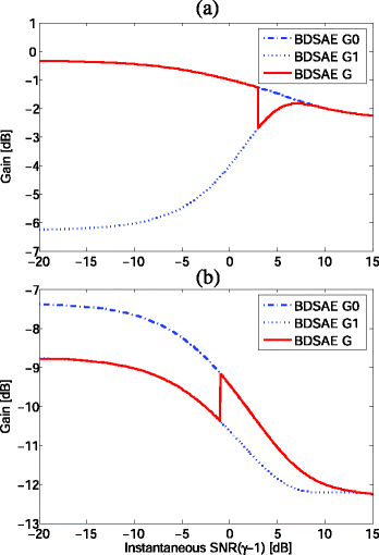

  

  Gains of Bayesian decision and estimation system versus instantaneous SNR (γ − 1). a System gain change from G ₀ to G ₁, for the case of p = 0.5, β = 0.5, and a priori SNR ξ = 5 dB. b System gain change from G ₁ to G ₀, for the case of p = −0.5, β = 1.5, and a priori SNR ξ = −5 dB

As shown in Fig. 2a, for a priori SNR of ξ = 5 dB, as long as the instantaneous SNR is higher than about 3 dB, the speech decision changes from η ₀ to η ₁, thus the optimal system gain G changes from G ₀ to G ₁. Similarly, as shown in Fig. 2b, for a priori SNR of ξ = −5 dB, as long as the instantaneous SNR is higher than about −1 dB, the speech decision changes from η ₁ to η ₀, thus the optimal system gain G changes from G ₁ to G ₀. Note that if there is an ideal speech detector, a more significantly non-continuous gain would be obtained. However, in the proposed BDSAE scheme, although the speech detector is not ideal, it is optimized to minimize the combined Bayesian risk function R, that is, the non-continuous system gain G of the proposed BDSAE is optimal, which could obtain good enhancement performance shown in Section 5.

• 4. Influence of cost parameters: In addition, from (23) we can see that, in the proposed BDSAE method, the non-continuous system gain G depends on the cost parameters c _ij as well as parameters p and β. If the cost parameter c ₀₁ associated with false alarm is much less than the generalized likelihood ratio Λ(Y(ω)), that is, the speech is definitely present in the spectral amplitude, the BDSAE gain function G ₁(ξ, γ, p, β) under the decision η ₁ can be approximated as follows:

$$ {G}_{\mathrm{appr}}\left(\xi, \gamma \right) \approx {\left(\frac{\left[{\left(\frac{\sqrt{v}}{\gamma}\right)}^{\beta}\varGamma \left(\frac{p+\beta }{2}+1\right)\varPhi \left(-\frac{p+\beta }{2},1;-v\right)\right]}{\left[\varGamma \left(\frac{p}{2}+1\right)\varPhi \left(-\frac{p}{2},1;-v\right)\right]}\right)}^{1/\beta } $$

(26)

In this way, the gain function G ₁(ξ, γ, p, β) is equal to G _appr(ξ, γ), which means a good enhancement effect can be obtained under correct decision η ₁. However, if the cost parameter c ₀₁ is much larger than the generalized likelihood ratio Λ(Y(ω)), the speech is absent in the spectral amplitude. In this case, the BDSAE gain function G ₁(ξ, γ, p, β) under the decision η ₁ (i.e., false alarm) is equal to G _f approximately (i.e., G ₁(ξ, γ, p, β) ≈ G _f ), and thus the cost of false alarm is compensated and the residual noise in the enhanced speech signals can be reduced effectively. On the other hand, if the cost parameter c ₁₀ associated with missed detection is much smaller than the inverse of generalized likelihood ratio Λ(Y(ω)), the BDSAE gain function G ₀(ξ, γ, p, β) under the decision η ₀ is equal to G _f approximately (i.e., G ₀(ξ, γ, p, β) ≈ G _f ). Therefore, it can remove noise greatly when speech is definitely absent. On the contrary, if the cost parameter c ₁₀ is much greater than the inverse of Λ(Y(ω)), the BDSAE gain function G ₀(ξ, γ, p, β) under the decision η ₀ (i.e., miss decision) is equivalent to the gain function G _appr(ξ, γ) of (26) (i.e., G ₀(ξ, γ, p, β) ≈ G _appr (ξ, γ)), so the cost of miss decision can be compensated and the speech distortion can be reduced as well. Here, in order to obtain a better trade-off between speech distortion and noise reduction, the empirical values of cost parameters c ₀₁ and c ₁₀ are chosen the same as 1.5.

• 5. Influence of p and β parameters: Furthermore, the p and β parameters are also more important to system gain G of the BDSAE method. Figure 3 shows their influences on gain function G _j (ξ, γ, p, β) for different p and β values, where the parameters c ₀₁ = 1.5, c ₁₀ = 5, q = 0.8, and G _f  = −15 dB, respectively. Here, the value of (γ − 1) is referred to as the instantaneous SNR.

  Fig. 3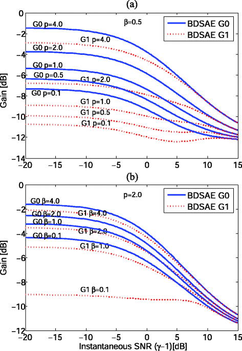

  

  Gains of BDSAE estimator versus instantaneous SNR (γ − 1) for different p and β values. a Gains versus instantaneous SNR (γ − 1) for different p values, for the case of β = 0.5 and a priori SNR ξ = −5 dB. b Gains versus instantaneous SNR (γ − 1) for different β values, for the case of p = 2 and a priori SNR ξ = −5 dB

As shown in Fig. 3a, given a fixed parameter β = 0.5 and the a priori SNR ξ = −5 dB, the gain G ₀ and G ₁ of BDSAE estimator always increase with the increasing of parameter p when instantaneous SNR (γ − 1) varies from −20 to 15 dB. That is, for different p values, we can obtain different system gain G values, and the corresponding noise reductions can be achieved.

From Fig. 3b, we can see that the gain G ₀ and G ₁ of BDSAE estimator also always increase with the increasing of parameter β for a fixed p = 2 and the a priori SNR ξ = −5 dB when instantaneous SNR (γ − 1) varies from −20 to 15 dB. Namely, for the different β values, the system gain G values are different, and the noise reduction obtained is also different. In this way, we can obtain the appropriate system gain G values by adaptively choosing the right p and β values, which can yield effective noise reduction and good speech enhancement performance. The adaptive calculation methods of p and β parameters will be presented in Section 3.

3 Adaptive calculation of p and β parameters

From the aforementioned analysis, we can see that the perceptually weighted order p and the spectral amplitude order β play an important role in speech enhancement, which can result in a better enhancement performance by choosing appropriate values for p and β. Therefore, in this section, we will present an adaptive calculation method for p and β, respectively.

3.1 Adaptive calculation of parameter p

For the calculation of parameter p, in [12], the method did not consider the variability of p, and just a fixed p value was chosen for the trade-off between noise reduction and speech distortion. Since no flexible gain was introduced, the enhancement performance of the estimator was limited. In [14], the variability of parameter p was considered, and an adaptive calculation method of p was presented, in which the parameter p was considered as a polynomial of the sub-band SNR and auditory perceptual parameter. In this way, for a larger STSA and a smaller STSA, the speech estimation errors can be penalized differently. However, the method shown in [14] needs to calculate the masking thresholds, and thus the pre-enhancement process is required, which increases the computational complexity greatly.

Since most of the speech energy is located at the lower frequencies (i.e., larger STSA) and at the higher frequencies, the speech energy is weakened (i.e., smaller STSA) [19], for the lower frequencies, the value of parameter p should be high and vice versa for the higher frequencies. That is, the estimation error at the higher frequencies is penalized more heavily than that at the lower frequencies. In this way, the residual noise can be suppressed effectively at the higher frequencies, and the speech distortion at the lower frequencies can be reduced at the same time. Therefore, on the basis of such idea, we propose a new adaptive calculation method for parameter p.

First, the appropriate lower bound and higher bound of parameter p for high frequency and low frequency require to be chosen, respectively. As discussed in [12], the p value with more negative produced more noise reduction but the greater speech distortion was introduced as well. Moreover, the p = −1 was suggested as a good trade-off between the noise reduction and speech distortion in [12]. Therefore, we choose p _min  = −1 as the lower bound of parameter p for high frequency. According to [14], in order to reduce the speech distortion at lower frequencies, p _max is set up to 4.0 as the upper bound of parameter p for low frequency in this paper.

Second, since the speech energy usually decreases as frequency increases, for the calculation of p value at the intermediate frequencies, the linear decreasing of p is proposed as a function of the frequency, i.e.,

$$ p(k)={p}_{\max }-\frac{k\left({p}_{\max }-{p}_{\min}\right)}{N} $$

(27)

where k is the index of frequency bins, N is the frame length, and p(k) denotes the p value of the kth frequency bin.

According to (27), we can obtain the decreased gain from lower frequency to higher frequency, and a larger noise reduction can be achieved at high frequencies, and thus the speech distortion at the higher frequencies is inevitable because the larger STSA sometimes exists at the higher frequencies. In order to reduce the speech distortion at the higher frequencies, we employ the sub-band SNR to modify p. First, the 21 critical sub-bands [20] are divided for each frame of noisy observation. Then the variable $\tilde{p}$ is assumed to be a linear function of the critical sub-band SNR Ξ(b, k), where b is the index of the critical bands. Finally, the range of $\tilde{p}$ is limited as [${\tilde{p}}_{\min }$, ${\tilde{p}}_{\max }$] to obtain a trade-off between the noise reduction and speech distortion [16]. In this way, the value of $\tilde{p}$ can be calculated by the following:

$$ \tilde{p}(k)= \max \left\{ \min \left[\mu \cdot \varXi \left(b,k\right)+\upsilon, {\tilde{p}}_{\max}\right],{\tilde{p}}_{\min}\right\} $$

(28)

where b denotes the index of the critical bands and k is the index of frequency bins. Ξ(b, k) denotes the kth sub-band SNR that belongs to the bth band. The constants μ and υ are set to 0.45 and 1.5, respectively, and the minimum and maximum values of $\tilde{p}$ are set to 0.4 and 4.0, respectively, i.e., ${\tilde{p}}_{\min }$ = 0.4 and ${\tilde{p}}_{\max }$ = 4.0.

According to (27) and (28), the final parameter p is obtained by weighting p and $\tilde{p}$:

$$ \widehat{p}(k)=\varepsilon \cdot \tilde{p}(k)+\left(1-\varepsilon \right)\cdot p(k) $$

(29)

where the weighting factor ε is related to the sub-band SNR Ξ(b, k), which is defined by the following:

$$ \varepsilon =\frac{1}{1+ \exp \left(-\left(\Xi \left(b,k\right)-{\Xi}_0\right)\right)} $$

(30)

where Ξ₀ is a constant. Here, Ξ₀ = 3.22 and Ξ(b, k) is defined as follows:

$$ \varXi \left(b,k\right)=\frac{{\displaystyle \sum_{k={B}_{\mathrm{low}}(b)}^{B_{\mathrm{up}}(b)}\left|Y\left(b,k\right)-\sqrt{\lambda_d\left(b,k\right)}\right|{}^2}}{{\displaystyle \sum_{k={B}_{\mathrm{low}}(b)}^{B_{\mathrm{up}}(b)}{\lambda}_d\left(b,k\right)}} $$

(31)

in which b denotes the index of the critical bands, k is the index of frequency bins. B _up(b) and B _low(b) denote the upper and lower frequency bound of the bth critical band, respectively. Y(b, k) denotes the kth spectral amplitude of noisy speech that belongs to the bth band, and λ _d (b, k) is the kth noise variances that belongs to the bth band.

3.2 Adaptive calculation of parameter β

For the calculation of β, in [15] and [16], the calculation methods of parameter β are based on overall SNR of each frame, and a linear relationship between β and frame SNR was applied. The β only monotonically increases or decreases with the frame SNR increases or decreases. That is, the value of β is fixed and does not vary with the frequency bins in each frame, so it cannot obtain flexible gain, the enhancement performance is limited. For this problem, a solution was proposed in [14], in which the parameter β was interpreted as the compression rate of the spectral amplitude and calculated based on the critical band. That is, the β value is different for different critical band, which can result in a more flexible gain. However, there is no consensus on the degree of compressive nonlinearity at the lower and intermediate frequencies, which might influence the accuracy of β value. Therefore, in this paper, we propose a new calculation method for the parameter β that varies with the frequency bins.

As we know, the higher the a posterior SNR γ(k) of (12), the larger the speech presence probability, so β should be larger for reducing speech distortion and vice versa. Therefore, according to γ(k), we can employ a monotonically increasing sigmoid function [21] to calculate the value of β.

First, since the strong correlation exists between the adjacent frequency bins, the average posterior SNR $\tilde{\gamma}(k)$ is obtained by applying a normalized window to γ(k),

$$ \tilde{\gamma}(k)={\displaystyle \sum_{i=-{L}_h}^{L_h}h(i)\gamma \left(k-i\right)} $$

(32)

where h is a normalized hamming window with length 2L _h  + 1 and L _h  = 5.

Second, the β value is often limited to the range of [0.001, 4.0] for the trade-off between noise reduction and speech distortion [14–16]. Therefore, the sigmoid function is employed to map the $\tilde{\gamma}(k)$ into (0, β _max) for parameter β, then we have

$$ \beta (k)=\frac{\beta_{\max }}{1+ \exp \left(-\alpha \left(\tilde{\gamma}(k)-{\gamma}_0\right)\right)} $$

(33)

where α is used to control the steepness of the sigmoid function, γ ₀ is the position of the inflection point, and β _max is a constant. They are set to 0.42, 3.5, and 4.0, respectively. And β(k) denotes the β value of the kth frequency bin.

Finally, we limit the minimum value of β to 0.001, that is, the final β is obtained by:

$$ \widehat{\beta}(k)= \max \left\{\beta (k),{\beta}_{\min}\right\} $$

(34)

where k is the index of frequency bins, β _min = 0.001. Figure 4 gives the variation of β values versus a posterior SNR γ(k).

Fig. 4

The variation of β values versus the a posterior SNR γ(k)

As shown in Fig. 4, the β value of the proposed method is a monotonically increasing function with respect to γ(k). Namely, the larger noise reduction can be yielded as γ(k) decreases, and the lower speech distortion can be achieved when γ(k) increases.

4 Implementation of the proposed method

In this section, we present the implementation of the proposed BDSAE method. The block diagram of the implementation is given in Fig. 5. Firstly, the noisy speech is windowed and transformed into frequency domain by DFT. Secondly, the minima controlled recursive averaging (MCRA) method [22] is employed to estimate the noise power spectrum. Thirdly, using the spectral amplitude of the noisy speech and the estimated noise power spectrum, the critical sub-band SNRs are obtained. Fourthly, the parameters p and β are adaptively calculated according to the critical sub-band SNRs and a posteriori SNRs. Finally, combining a posteriori SNR and a priori SNR obtained by a decision-directed (DD) method [5], the optimal spectral amplitude estimator and decision rule of the BDSAE method are derived by further minimizing the combined Bayesian risk function R, which are used to enhance DFT coefficients of the noisy speech. Then the inverse Fourier transform and the overlap-adding algorithm are performed to obtain the enhanced speech signal in the time domain.

Fig. 5

The block diagram of the proposed method

5 Performance evaluation

In this section, we discuss the performance evaluation of the proposed BDSAE method. First, the experimental setup of the proposed method is described. Then, we compare the objective and subjective experimental results between the proposed method and the reference methods.

5.1 Experimental setup

In order to evaluate the performance of the proposed BDSAE method for speech enhancement, white Gaussian noise, street noise, and interior Volvo car noise from ITU-T noise database and babble noise, factory noise, and Fl6 cockpit noise from NOISEX-92 [23] database were used in the test experiments. Twenty-four speech sentences were taken from the Chinese sub-database of NTT speech database, where 12 sentences produced by two female speakers (i.e., six sentences for each female speaker) and another 12 sentences produced by two male speakers (i.e., six sentences for each male speaker). All these speech signals and noises are re-sampled at 16 kHz, and all the signals were 8 s in duration. Frame size N is 512 samples, and the samples are sine windowed with 50 % overlap between adjacent frames. The noisy speech signals were produced according to ITU-T P.56 standard [24], and the input SNRs of noisy speech are 0, 5, 10, and 15 dB, respectively.

In the experiments, the MMSE STSA estimator [5], the SDEA estimator [11], the weighted Euclidean distortion measure (WEDM) estimator [12], and the β-STSA estimator [16] are chosen as the reference methods for comparing with the proposed BDSAE method. The DD method [5] is applied to all these reference methods and the BDSAE method. The MCRA algorithm [22] is used for these methods to estimate noise power spectrum from noisy speech signals. All the reference methods we used were implemented according to the referenced papers, and the corresponding parameters of the methods were not tuned as well.

For the performance evaluation of the speech enhancement methods, the segmental SNR (SNR_seg) measure [25], the log-spectral distortion (LSD) measure [11], and the perceptual evaluation of speech quality (PESQ) [26] were used as objective quality evaluation methods. Furthermore, the Multiple Stimuli with Hidden Reference and Anchor (MUSHRA) listening test [27] was employed to evaluate the subjective quality.

5.2 Objective quality tests

In this subsection, we describe various objective quality tests. Before we provide rigorous quantitative results, we briefly discuss spectrograms of the signals processed by the proposed system and the reference systems.

• 1. Spectrograms: Figure 6 shows the spectrograms of the input noisy speech (mixed with white Gaussian noise for 0 dB) and the enhanced speech signals obtained by the various enhancement methods. From Fig. 6, we can see that the proposed method outperforms the reference methods.

  Fig. 6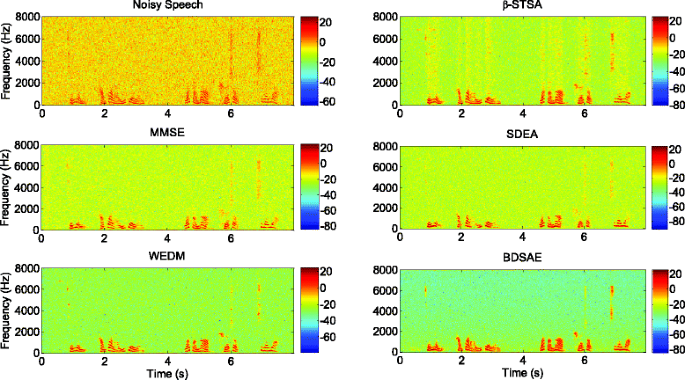

  

  The speech spectrogram comparison for the various enhancement methods

• 2. Segmental SNR: The SNR_seg [25] measure can be employed to evaluate the objective quality of enhanced speech signals of different speech enhancement methods. The SNR_seg is measured by calculating the SNR for each frame of speech and averaging these SNRs over all test speech sequences, which can be defined by the following:

$$ SN{R}_{\mathrm{seg}}=\frac{1}{L}{\displaystyle \sum_{l=0}^{L-1}10\cdot { \log}_{10}}\left(\frac{{\displaystyle {\sum}_{n=Nl}^{Nl+N-1}{x}^2(n)}}{{\displaystyle {\sum}_{n=Nl}^{Nl+N-1}{\left[x(n)-\widehat{x}(n)\right]}^2}}\right) $$

(35)

where n denotes the index of signal samples, N is the frame length. l is frame index, and L is the total number of frames. x(n) denotes the clean speech signal, and $\widehat{x}(n)$ denotes the enhanced speech signal.

For different input SNRs (i.e., 0, 5, 10, and 15 dB), Fig. 7 gives the comparison of SNR_seg improvement for different enhancement methods under White Gaussian noise. Figure 8 gives the comparison of SNR_seg improvement for different enhancement methods under factory noise.

Fig. 7

Comparison of SNR_seg improvement under White Gaussian noise

Fig. 8

Comparison of SNRseg improvement under factory noise

From Figs. 7 and 8, we can see that, in the case of white Gaussian noise and Factory noise, the SNR_seg improvement of the WEDM method is much better than the other reference methods, but a little worse than the proposed BDSAE method. The SNR_seg improvements of the BDSAE method are nearly 5.0 and 3.0 dB larger than the WEDM method in the white Gaussian noise and factory noise conditions, respectively.

For each input SNR, the average SNR_seg improvement of various enhancement methods for six types of noise are presented in Table  1 .

Table 1 Test results of SNRseg improvement

From Table  1 , we can find that BDSAE method produce much higher average SNR_seg improvement than the reference methods. Furthermore, for each input SNR, in comparison with the WEDM method whose performance is better than the other reference methods, the average SNR_seg improvement of the BDSAE method is increased about 3.3 dB for all test noise signals. Therefore, according to the experimental results of Figs. 7 and 8 and Table  1 , it is obvious that the BDSAE method performs better than the reference methods.

• 3. LSD: The LSD measure [11] is also used to evaluate the objective quality of the enhanced speech, which measures the similarity between the clean speech spectrum and the estimated speech spectrum. The definition of LSD is given as:

$$ {d}_{\mathrm{LSD}}=\frac{1}{L}{\displaystyle \sum_{l=0}^{L-1}\sqrt{\frac{1}{N}{\displaystyle \sum_{k=0}^{N-1}{\left[10{ \log}_{10}\frac{\left|\widehat{X}\left(l,k\right)\right|{}^2}{\left|X\left(l,k\right)\right|{}^2}\right]}^2}}} $$

(36)

where l is the frame index, k is the index of frequency bins, L is the total frames, and N is the frame length. X(l, k) denotes the DFT coefficient of the clean speech signal and $\widehat{X}\left(l,k\right)$ denotes the DFT coefficient of the enhanced speech signal.

According to the idea of [11], the log-spectrum dynamic range of speech signal is confined to about 50 dB for the LSD experiments. The LSD test results are shown in Figs. 9 and 10 for the case of white Gaussian noise and factory noise, respectively. The average LSD test results are given in Table  2 for different input SNRs.

Fig. 9

Comparison of LSD under white Gaussian noise

Fig. 10

Comparison of LSD under factory noise

Table 2 Test results of LSD

From Figs.  9 and 10 , we can see that, in the white Gaussian noise and Factory noise conditions, all speech enhancement methods can obviously reduce the LSD comparing with the noisy speech, where the BDSAE method can obtain much lower LSD than the other reference methods for four SNR conditions. By comparing with the WEDM method whose LSD is lower than the other reference methods, the average LSDs of the BDSAE method are decreased about 3.0 and 1.5 dB for different input SNRs in the white Gaussian noise and factory noise conditions, respectively.

From Table  2 , we can see that, by comparing with the LSD of noisy speech, all speech enhancement methods can reduce the LSD to some extent. The average LSD of the BDSAE method is lower than the reference methods in various input SNRs. That is, the proposed method outperforms the reference methods.

• 4. PESQ: The PESQ [26] is widely used to assess the objective quality of speech signals, and a higher PESQ score corresponds to a better speech quality. For the case of white Gaussian noise and factory noise, the PESQ test results are compared in Figs. 11 and 12, respectively. The total average PESQ scores of six types of noise are given in Table  3 for four kinds of input SNRs.

  Fig. 11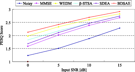

  

  Comparison of PESQ under White Gaussian noise

  Fig. 12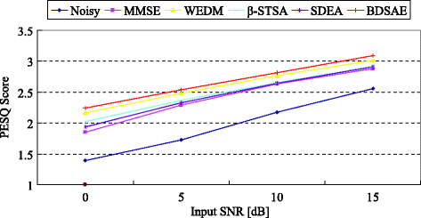

  

  Comparison of PESQ under factory noise

  Table 3 Test results of PESQ

From Figs. 11 and 12, we can see that, for the case of white Gaussian noise and Factory noise, in comparison with the reference methods, the BDSAE method yields higher average PESQ scores for various input SNR conditions.

From Table  3 , we can find that the average PESQ scores of the enhanced speech signals are all higher than noisy speech signals, which illustrates that the quality of enhanced speech signals produced by all kinds of enhancement methods are improved obviously. In addition, by comparing with the reference methods, the BDSAE method produces higher average PESQ scores for various input SNR conditions. Therefore, it is further confirmed that the proposed BDSAE method is superior to the reference algorithms.

5.3 Subjective quality tests

The quality of enhanced speech is generally assessed by subjective perception, such as speech intelligibility, naturalness, and articulation. The MUSHRA listening test [27] is a commonly used method for the subjective evaluation of audio quality. It requires fewer participants to obtain a statistically significant result [27] reference. Therefore, we employed the MUSHRA listening test to evaluate the subjective quality of enhanced speech. In the MUSHRA test, the subjects are provided with the signals under test as well as one reference and a hidden anchor. The subjects are asked to grade the different signals on a quality scale between 0 and 100, 100 being the best score. As the hidden anchor, we used a speech signal having an SNR of 5 dB less than the noisy speech to be enhanced [20]. The listeners were allowed to listen to each test speech several times and always had access to the clean speech reference.

Six male and four female listeners whose ages are from 20 to 30 years old participated in the MUSHRA tests. Two speech sentences (i.e., one male speaker, one female speaker) were randomly chosen from the aforementioned twenty-four speech sentences, and the corresponding noisy speech sentences contaminated by the aforementioned six types of noise under the different input SNRs (i.e., 0, 5, 10, and 15 dB) were chosen from noisy speech data set which is discussed in Section 5.1. All these noisy speeches were enhanced by the speech enhancement methods and were used for the MUSHRA test. After all the listeners had graded the test signals, a statistical analysis of the results was conducted for the different speech enhancement methods for different input SNRs. Figure 13 shows the MUSHRA listening test results, with the average MUSHRA scores together with the 95 % confidence intervals.

Fig. 13

Comparison of the MUSHRA score

From Fig. 13, we can find that, for four input SNR conditions, the WEDM method yields higher average MUSHRA scores than the other reference methods but lower than the BDSAE method. That is, the proposed BDSAE method performs better than the state-of-the-art reference methods for the subjective quality.

5.4 Discussion

From the aforementioned experimental results, we can see that the proposed BDSAE approach performs better than the reference methods. Herein, we discuss its advantages to the reference methods.

As we know, the spectral amplitudes of speech signal are generally sparse since only some frequency bins contain significant energy in each speech frame. However, the reference methods do not take the sparse characteristics into consideration and often only focus on estimating the speech spectral amplitude rather than detecting their existence in the frequency bins. In this way, for the speech presence or speech absence in the frequency bins, they only use the same gain function to estimate clean speech from noisy speech, which limits their enhancement performance.

For the proposed BDSAE approach, the sparse characteristics of spectral amplitudes of speech signal are considered. That is, under speech presence or speech absence in frequency bins, the cost functions are different which result in different gain functions. Then the speech detector is derived to choose the optimal gain function to estimate clean speech. In this way, for speech presence or speech absence in frequency bins, the gain functions are different and optimal, respectively, which can yield better speech enhancement performance. Moreover, the speech distortion and residual noise resulted from the detector error (i.e., missed detection and false alarm) can be compensated by cost parameters c _ij , which is discussed in Section 2.3 (i.e., (4) Influence of cost parameters).

In addition, the p and β parameters are induced to cost functions of the BDSAE approach, and the values of p and β are adaptive calculation as the frequency bins. Therefore, we can obtain more flexible and effective gain functions under speech presence and speech absence in frequency bin, which can yield effective noise reduction and good speech enhancement performance.

As can be seen from (23), the proposed BDSAE approach requires the calculation of two gain functions, G ₀ and G ₁, and the decision rule, in which the mainly computational complexity is focus on calculating the gamma function Г(∙) and the confluent hyper-geometric function Ф(∙). However, for the four reference methods (i.e., MMSE, WEDM, β-STSA, and SDEA) listed in Section 5.1, they also require to calculate the two functions of Г(∙) and Ф(∙). Therefore, the computational complexity of the proposed BDSAE approach is at the same level compared to the four reference methods. In addition, the proposed BDSAE approach is implemented frame by frame, and thus, there is no any delay existed.

To implement the proposed BDSAE method for real-time realization, the computational complexity involved in (23) could be further simplified. Here, we apply the idea of looking up a table [14, 16] for simplifying the gain function G _j (ξ, γ, p, β) of (23). For the numerator and the denominator of (23), the algebraic product of the gamma function Γ(.) and the confluent hyper-geometric function Φ(.) can be considered as the function of variables φ and ν, namely, Ψ(φ, ν) = Γ(φ + 1)Φ(−φ, 1; ν). The variable φ is the function of parameters p and β in the BDSAE estimator, i.e., φ ₁ = (p + β)/2, φ ₂ = p/2. In this way, the gain function G _j (ξ, γ, p, β) of Eq. (23) can be simplified as follows:

$$ {G}_j\left(\zeta, \gamma, p,\beta \right)={\left(\frac{c_{1j}\varLambda \left(Y\left(\omega \right)\right){\left(\raisebox{1ex}{$\sqrt{v}$}\!\left/ \!\raisebox{-1ex}{$\gamma $}\right.\right)}^{\beta}\varPsi \left({\varphi}_1,-v\right)+{c}_{0j}{G}_f^{\beta }}{c_{1j}\varLambda \left(Y\left(\omega \right)\right)\varPsi \left({\varphi}_2,-v\right)+{c}_{0j}}\right)}^{\raisebox{1ex}{$1$}\!\left/ \!\raisebox{-1ex}{$\beta $}\right.} $$

Therefore, according to [14] and [16], the Ψ(φ, ν) is designed for looking up a table which relies on variables φ and ν. The computational complexity of the proposed method is reduced greatly by the above simplification.

6 Conclusions

We present a single-channel speech enhancement method based on BDSAE. The optimal speech decision rule and spectral amplitude estimator are derived by jointly minimizing the combined Bayesian risk function which considers both detection and estimation errors. Under presence and absence of spectral amplitude, the general weighted cost function is proposed, in which the perceptually weighted order p and the spectral amplitude order β are jointly used. In order to obtain flexible gain values for the BDSAE method, the adaptive estimation methods for the p and β parameters are presented, respectively. Furthermore, the cost parameters in the cost function are employed to balance the speech distortion and residual noise caused by missed detection and false alarm, respectively. Therefore, the BDSAE method not only considers the sparse characteristics of the spectral amplitudes of speech signal but also takes the full advantages of both the traditional perceptual weighted estimators and β-order spectral amplitude estimators, which can obtain more flexible and effective gain functions. Finally, we took the objective and subjective quality tests for the enhanced speech based on SNR_seg, LSD, PESQ, and MUSHRA listening tests, respectively. The test results indicate that the proposed BDSAE method can achieve a more significant performance improvement than the reference methods.

Appendices

Appendix 1—the derivation procedure of r _1j (Y(ω _k )) of Eq. (24)

In this appendix, we derive the r _1j (Y(ω _k )) of Eq. (24) and ignore the frequency bin k for notation simplification. Under speech hypothesis H ₁, by substituting speech presence cost function d _1j (X, $\widehat{X}$) into r _1j (Y(ω)) of (9), we can obtain

$$ {r}_{1j}\left(Y\left(\omega \right)\right)={c}_{1j}{\displaystyle \underset{\varOmega_x}{\int }{X}^p{\left({X}^{\beta }-{\left({G}_jY\right)}^{\beta}\right)}^2p\left(X\Big|{H}_1\right)p\left(Y\left(\omega \right)\Big|X\right)dX} $$

(37)

where we just call G _j (ξ, γ, p, β) as G _j for convenience and $\widehat{X}={G}_jY$.

According to [28], we can get the multiplication of the two probability density functions as follows:

$$ p\left(X\Big|{H}_1\right)p\left(Y\left(\omega \right)\Big|X\right)={\displaystyle \underset{0}{\overset{2\pi }{\int }}p\left(x,\theta \Big|{H}_1\right)p\left(Y\left(\omega \right)\Big|x,\theta \right)d\theta } $$

(38)

where x is the implementation of amplitude variable X and θ is the implementation of phase variable of X(ω). In this way, the (37) can be rewritten as follows:

$$ {r}_{1j}\left(Y\left(\omega \right)\right)={c}_{1j}{\displaystyle \underset{0}{\overset{\infty }{\int }}{\displaystyle \underset{0}{\overset{2\pi }{\int }}{x}^p{\left({x}^{\beta }-{\left({G}_jY\right)}^{\beta}\right)}^2p\left(x,\theta \Big|{H}_1\right)p\left(Y\left(\omega \right)\Big|x,\theta \right) d\theta dx}} $$

(39)

where the probability density functions of (39) can be defined as follows [28]:

$$ p\left(x,\theta \Big|{H}_1\right)=\frac{x}{\pi {\lambda}_x} \exp \left(-\frac{x^2}{\lambda_x}\right) $$

(40)

$$ p\left(Y\left(\omega \right)\Big|x,\theta \right)=\frac{1}{\pi {\lambda}_d} \exp \left(-\frac{\left|Y\left(\omega \right)-X\left(\omega \right)\right|{}^2}{\lambda_d}\right) $$

(41)

By applying the two probability density functions of (40) and (41), we can obtain

$$ \begin{array}{l}p\left(x,\theta \Big|{H}_1\right)p\left(Y\left(\omega \right)\Big|x,\theta \right)\\ {}\kern1.25em =\frac{x}{\pi^2{\lambda}_x{\lambda}_d} \exp \left(-\left(\gamma +\frac{x^2}{\lambda_x}-\frac{2Yx \cos \left(\theta -{\theta}^{\hbox{'}}\right)}{\lambda_d}\right)\right)\end{array} $$

(42)

According to [11, 29], we have

$$ {\displaystyle \underset{0}{\overset{2\pi }{\int }} \exp \left(\frac{2Yx \cos \left(\theta -{\theta}^{\hbox{'}}\right)}{\lambda_d}\right)d}\theta =2\pi {J}_0\left(i\frac{2Y}{\lambda_d}x\right) $$

(43)

where J ₀(.) denotes the zero-order Bessel function.

By substituting (42) and (43) into (39), we can get

$$ \begin{array}{l}{r}_{1j}\left(Y\left(\omega \right)\right)=\frac{2{c}_{1j} \exp \left(-\gamma \right)}{\pi {\lambda}_x{\lambda}_d}{\displaystyle \underset{0}{\overset{\infty }{\int }}{x}^{p+1}{\left({x}^{\beta }-{\left({G}_jY\right)}^{\beta}\right)}^2 \exp \left(-\frac{x^2}{\lambda_x}\right){J}_0\left(i\frac{2Y}{\lambda_d}x\right)}dx\\ {}=\frac{2{c}_{1j} \exp \left(-\gamma \right)}{\pi {\lambda}_x{\lambda}_d}{\displaystyle \underset{0}{\overset{\infty }{\int }}\left[{x}^{2\beta +p+1}+{x}^{p+1}{\left({G}_jY\right)}^{2\beta }-2{x}^{\beta +p+1}{\left({G}_jY\right)}^{\beta}\right] \exp \left(-\frac{x^2}{\lambda_x}\right){J}_0\left(i\frac{2Y}{\lambda_d}x\right)}dx\end{array} $$

(44)

where λ _x and λ _d are the speech and noise variances and γ is a posteriori SNR.

Simplifying (44), we obtain

$$ {r}_{1j}\left(Y\left(\omega \right)\right)=\frac{2{c}_{1j} \exp \left(-\gamma \right)}{\pi {\lambda}_x{\lambda}_d} \cdot \left[\begin{array}{l}{\displaystyle \underset{0}{\overset{\infty }{\int }}{x}^{2\beta +p+1} \exp \left(-\frac{x^2}{\lambda_x}\right){J}_0\left(i\frac{2Y}{\lambda_d}x\right)}dx\\ {}+{\left({G}_jY\right)}^{2\beta }{\displaystyle \underset{0}{\overset{\infty }{\int }}{x}^{p+1} \exp \left(-\frac{x^2}{\lambda_x}\right){J}_0\left(i\frac{2Y}{\lambda_d}x\right)}dx\\ {}-2{\left({G}_jY\right)}^{\beta }{\displaystyle \underset{0}{\overset{\infty }{\int }}{x}^{\beta +p+1} \exp \left(-\frac{x^2}{\lambda_x}\right){J}_0\left(i\frac{2Y}{\lambda_d}x\right)}dx\end{array}\right] $$

(45)

Following ([29], eq. 6.631.1), we have

$$ \begin{array}{l}{\displaystyle \underset{0}{\overset{\infty }{\int }}{x}^{\mu } \exp \left(-a{x}^2\right){J}_v(bx)dx}\\ {}\kern0.5em =\frac{b^v\varGamma \left(0.5v+0.5\mu +0.5\right)}{2^{v+1}{a}^{0.5\left(v+\mu +1\right)}\varGamma \left(v+1\right)}\varPhi \left(\frac{\mu +v+1}{2},v+1;-\frac{b^2}{4a}\right)\end{array} $$

(46)

By substituting (46) into (45), we can obtain (47) which is the same with (24).

$$ {r}_{1j}\left(Y\left(\omega \right)\right)=\frac{c_{1j} \exp \left(-\frac{\gamma }{1+\xi}\right)}{\pi {\lambda}_d\left(1+\xi \right)} \cdot \left[\begin{array}{l}{\phi}^{\left(p/2+\beta \right)}\varGamma \left(\frac{p}{2}+\beta +1\right)\varPhi \left(-\left(\frac{p}{2}+\beta \right),1;-v\right)\\ {}+{\left({G}_jY\right)}^{2\beta }{\phi}^{\left(p/2\right)}\varGamma \left(\frac{p}{2}+1\right)\varPhi \left(-\frac{p}{2},1;-v\right)\\ {}-2{\left({G}_jY\right)}^{\beta }{\phi}^{\left(p/2+\beta /2\right)}\varGamma \left(\frac{p+\beta }{2}+1\right)\varPhi \left(-\frac{p+\beta }{2},1;-v\right)\end{array}\right] $$

(47)

Appendix 2—the derivation procedure of r _0j (Y(ω)) of Eq. (25)

In this appendix, we derive the r _0j (Y(ω)) of Eq. (25) and call G _j (ξ, γ, p, β) as G _j for convenience. Under hypothesis H ₀, by substituting speech absence cost function d _0j (X, $\widehat{X}$) into r _0j (Y(ω)) of (9), we can obtain

$$ {r}_{0j}\left(Y\left(\omega \right)\right)={c}_{0j}{\displaystyle \underset{0}{\overset{\infty }{\int }}{\left({\left({G}_fY\right)}^{\beta }-{\left({G}_jY\right)}^{\beta}\right)}^2p\left(X\Big|{H}_0\right)p\left(Y\left(\omega \right)\Big|X\right)}dX $$

(48)

Following (7), we have p(X|H ₀) = δ(X). Then the Dirac delta function is substituted into (48), we can obtain

$$ {r}_{0j}\left(Y\left(\omega \right)\right)={c}_{0j}{\left({\left({G}_fY\right)}^{\beta }-{\left({G}_jY\right)}^{\beta}\right)}^2p\left(Y\left(\omega \right)\Big|{H}_0\right) $$

(49)

According to [28], the p(Y(ω)|H ₀) of (49) can be defined as:

$$ p\left(Y\left(\omega \right)\Big|{H}_0\right)=\frac{1}{\pi {\lambda}_d} \exp \left(-\frac{Y^2}{\lambda_d}\right) $$

(50)

where λ _d denotes the variance of noise signal.

By substituting (50) into (49), we can obtain (51) which is (25).

$$ \begin{array}{l}{r}_{0j}\left(Y\left(\omega \right)\right)={c}_{0j}{\left({\left({G}_fY\right)}^{\beta }-{\left({G}_jY\right)}^{\beta}\right)}^2\frac{1}{\pi {\lambda}_d} \exp \left(-\frac{Y^2}{\lambda_d}\right)\\ {}\kern4em =\frac{c_{0j}}{\pi {\lambda}_d}{\left({G}_f^{\beta }-{G}_j^{\beta}\right)}^2{Y}^{2\beta } \exp \left(-\gamma \right)\end{array} $$

(51)

References

SF Boll, Suppression of acoustic noise in speech using spectral subtraction [J]. IEEE Trans. Acoust., Speech Signal Process 27(2), 113–120 (1979)
DL Donoho, De-noising by soft-thresholding [J]. IEEE Trans. Inf. Theory 41, 613–627 (1995)
Y Ephraim, HL Van Trees, A signal subspace approach for speech enhancement [J]. IEEE Trans. Speech Audio Process. 3(4), 251–266 (1995)
N Virag, Single channel speech enhancement based on masking properties of the human auditory system [J]. IEEE Trans. Speech Audio Process. 7(2), 126–137 (1999)
Y Ephraim, D Malah, Speech enhancement using a minimum mean-square error short-time spectral amplitude estimator [J]. IEEE Trans. Acoust. Speech Signal Process 32, 1109–1121 (1984)
Y Ephraim, D Malah, Speech enhancement using a minimum mean-square error log-spectral amplitude estimator [J]. IEEE Trans. Acoust. Speech Signal Process 33, 443–445 (1985)
Malah, D., Cox, R. V., Accardi, A. J., Tracking speech-presence uncertainty to improve speech enhancement in non-stationary noise environments [A]. In Proc. 24th IEEE Int. Conf. Acoust., Speech, Signal Process., ICASSP’99 [C], Phoenix, AZ, 1999: 789–792.
I Cohen, B Berdugo, Speech enhancement for non-stationary environments [J]. Signal Process. 81, 2403–2418 (2001)
M Fujimoto, S Watanabe, T Nakatani, Frame-wise model re-estimation method based on Gaussian pruning with weight normalization for noise robust voice activity detection [J]. Speech Comm. 54(2), 229–244 (2012)
CH Hsieh, TY Feng, PC Huan, Energy-based VAD with grey magnitude spectral subtraction [J]. Speech Comm. 51(9), 810–819 (2009)
A Abramson, I Cohen, Simultaneous detection and estimation approach for speech enhancement [J]. IEEE Trans. Speech Audio Process. 15, 2348–2359 (2007)
P Loizou, Speech enhancement based on perceptually motivated Bayesian estimators of the speech magnitude spectrum [J]. IEEE Trans. Speech Audio Process. 13(5), 857–869 (2005)
Deng, F., Bao, C. C., Bao, F., A speech enhancement method by coupling speech detection and spectral amplitude estimation [A]. 14th Annual Conference of the International Speech Communication Association, Interspeech [C], Lyon, France, 2013: 3234–3238.
F Deng, F Bao, CC Bao, Speech enhancement using generalized weighted β-order spectral amplitude estimator [J]. Speech Comm. 59, 55–68 (2014)
CH You, SN Koh, S Rahardja, Masking-based β-order MMSE speech enhancement [J]. Speech Comm. 48(1), 57–70 (2006)
CH You, SN Koh, S Rahardja, β-order MMSE spectral amplitude estimation for speech enhancement [J]. IEEE Trans. Speech Audio Process. 13(4), 475–486 (2005)
A Fredriksen, D Middleton, D Vandelinde, Simultaneous signal detection and estimation under multiple hypotheses [J]. IEEE Trans. Inf. Theory 18(5), 607–614 (1968)
AG Jaffer, SC Gupta, Coupled detection-estimation of Gaussian processes in Gaussian noise [J]. IEEE Trans. Inf. Theory 18(1), 106–110 (1972)
E Plourde, B Champagne, Auditory-based spectral amplitude estimators for speech enhancement [J]. IEEE Trans. Speech Audio Process. 16(8), 1614–1623 (2008)
JD Johnston, Transform coding of audio signal using perceptual noise criteria [J]. IEEE J. Select. Areas Comm. 6, 314–323 (1988)
Fu Z. H., Wang J. F., Speech presence probability estimation based on integrated time-frequency minimum tracking for speech enhancement in adverse environments [A]. IEEE Int. Conf. Acoust., Speech, Signal Process., ICASSP [C], Dallas, Texas, USA, 2010: 4258–4261.
I Cohen, B Berdugo, Noise estimation by minima controlled recursive averaging for robust speech enhancement [J]. IEEE Signal Processing Letters 9(1), 12–15 (2002)
A Varga, H Steeneken, Assessment for automatic speech recognition: II. NOISEX-92: a database and an experiment to study the effect of additive noise on speech recognition systems [J]. Speech Comm. 12(3), 247–251 (1993)
ITU-T, Recommendation P.56: Objective measurement of active speech level, 1993.
SR Quackenbush, TP Barnwell, MA Clements, Objective measures of speech quality [J] (Englewood Cliffs, NJ, Prentice Hall, 1988)
ITU-T, Recommendation P.862: Perceptual evaluation of speech quality (PESQ), an objective method for end-to-end speech quality assessment of narrow-band telephone networks and speech codecs, 2001.
E. Vincent, 2005. MUSHRAM: a MATLAB interface for MUSHRA listening tests. [Online] http://www.elec.qmul.ac.uk/people/emmanuelv/mushram.
Loizou PC, Speech enhancement: theory and practice [M]. Boca Raton: CRC Press; 2007. 213–225.
IS Gradshteyn, IM Ryzhik, Table of integrals, series, and products [M], 6th edn. (Academic, New York, 2000)
Acknowledgements
This work was supported by the National Natural Science Foundation of China (Grant No. 61471014).
Author information
Authors and Affiliations
Corresponding author
Additional information
Competing interests
The authors declare that they have no competing interests.