Emotional voice conversion using neural networks with arbitrary scales F0 based on wavelet transform

Abstract

An artificial neural network is an important model for training features of voice conversion (VC) tasks. Typically, neural networks (NNs) are very effective in processing nonlinear features, such as Mel Cepstral Coefficients (MCC), which represent the spectrum features. However, a simple representation of fundamental frequency (F0) is not enough for NNs to deal with emotional voice VC. This is because the time sequence of F0 for an emotional voice changes drastically. Therefore, in our previous method, we used the continuous wavelet transform (CWT) to decompose F0 into 30 discrete scales, each separated by one third of an octave, which can be trained by NNs for prosody modeling in emotional VC. In this study, we propose the arbitrary scales CWT (AS-CWT) method to systematically capture F0 features of different temporal scales, which can represent different prosodic levels ranging from micro-prosody to sentence levels. Meanwhile, the proposed method uses deep belief networks (DBNs) to pre-train the NNs that then convert spectral features. By utilizing these approaches, the proposed method can change the spectrum and the F0 for an emotional voice simultaneously as well as outperform other state-of-the-art methods in terms of emotional VC.

1 Introduction

Recently, the study of voice conversion (VC) has attracted wide attention in the field of speech processing. This technology can be applied in various domains, such as emotion conversion [1], speech assistance [2], and other applications [3, 4]. Therefore, it has continued to motivate related studies each year. Many statistical approaches have been proposed for spectral conversion in the past few decades [5, 6]. Among these approaches, a Gaussian Mixture Model (GMM) has been commonly used, and many improvements have been proposed [7, 8] for GMM-based VC. Other VC methods, such as those based on non-negative matrix factorization (NMF) [2, 9], have also been proposed. The NMF and GMM methods are based on linear functions. For better VC performance, the VC technique needs to train more complex nonlinear features, such as Mel Cepstral Coefficients (MCC) [10], which are widely used in automatic speech and speaker recognition. Meanwhile, some approaches construct non-linear mapping relationships using neural networks (NNs) to train the mapping dictionaries between the source and target features [11], whereas others use deep belief networks (DBNs) to achieve non-linear deep transformation [12]. Results have shown that these deep architecture models have better performance than shallow conversion in some complex voice feature conversion.

However, most of the VC-related works focus on the conversion of spectral features, rather than on the conversion of fundamental frequency (F0). The spectral and F0 features obtained from STRAIGHT [13] can affect the voice’s acoustic and emotional features, respectively. F0 features comprise one of the most important parameters for representing emotional speech, because they can clearly describe the variation of voice prosody from one pitch period to another. However, F0 features extracted from STRAIGHT are low-dimensional features that cannot be processed well by deep models, such as NMF models or DBN models. Therefore, F0 features are usually converted by logarithm Gaussian (LG) normalized transformation [14] in these models. However, previous studies have shown that prosody conversion is affected by both short- and long-term dependencies, such as the sequence of segments, syllables, words within an utterance, as well as lexical and syntactic systems of a language [15]. The LG-based method is insufficient to convert the prosody effectively owing to constraints of their linear models and low-dimensional F0 features. In our earlier work [16], we proposed a new NN-based method that can train the segmental F0 features for emotional prosody conversion. Although we conducted segmental processing to increase the dimensions of F0 features that can be trained by the NNs well, the segmental F0 features cannot model F0 in different temporal scales. Continuous wavelet transform (CWT) can effectively model F0 in different temporal scales and significantly improve the speech synthesis performance [17]. For this reason, Suni et al. [18] applied CWT for intonation modeling in hidden Markov model (HMM) speech synthesis. Ming et al. [19] used CWT in F0 modeling within the NMF model for emotional VC and obtained a better result than the LG method in terms of F0 conversion. In their recent work [20], a deep learning model was used for F0 modeling in emotional VC.

In our recent work [21], inspired by the ability of deep learning models to perform well in complex non-linear feature conversion [12] and the ability of CWT to improve F0 feature conversion [19], we proposed a novel method that used NNs to train the CWT- F0 for converting the prosody of the emotional voice. Different from [19], we decomposed the F0 into 30 temporal scales containing more specifics of different temporal scales, and trained them by NNs, which can perform better compared with the LG model and the NMF-based model. In the current paper, we extend our earlier work [21] to systematically capture the F0 features of different temporal scales, which can then represent different prosodic levels ranging from micro-prosody to the sentence levels. We achieve this by using the CWT method to decompose the F0 contour into several temporal scales. This approach is different from our earlier research in [21], in which we decomposed the F0 with 30 discrete scales, each separated by one third of an octave.

In the current study, we proposed an arbitrary scales CWT (AS-CWT) method to decompose F0 to several scales, which can more approximately represent each level of individual prosodics. Given that the DBNs can effectively perform spectral envelope conversion, we train the MCC features for spectral feature conversion by using DBNs proposed by Nakashika et al. [12]. We chose different models to separately convert the spectral features and F0 feature. This is because, although the wavelet transform decomposed F0 features to more complex features, they can be trained enough by NNs, whereas the more complex spectral features require a deeper architecture. In the remaining part of this paper, we describe features processing concerning MCC and CWT in Section 2. The DBNs and NNs used in our proposed method are introduced in Section 3. In Section 4, we describe the framework of our proposed emotional VC system. Section 5 gives the detailed stages process of experimental evaluations, and Section 6 presents the conclusions.

2 Feature extraction and processing

The STRAIGHT is frequently used to extract features from a speech signal. Generally, the smoothing spectrum and instantaneous-frequency-based F0 are derived as excitation features for every 5 ms from the STRAIGHT [13]. To obtain the same number of frames, a dynamic time warping method is used to align the extracted features (spectrum and F0) of the source voice and target voice. Then, the aligned spectral features are translated into MCC. The F0 features produced by STRAIGHT are one dimensional and discrete. Modeling the variations of F0 in all temporal scales using linear models is difficult. Inspired by the work in [18], before training the F0 features by NNs, we adopted CWT to decompose the F0 contour into several temporal scales, which can then be used to model different prosodic levels ranging from micro-prosody to the sentence levels. In an earlier work [21], we adopted CWT to decompose the F0 contour into 30 temporal scales before training the F0 features by NNs. The decomposed 30 dimensional features are linearly spaced scales, each separated by one third of an octave. However, only the features that can represent the utterance, phrase, word, syllable, and phone levels are useful for training. Thus, in the current paper, we apply the AS-CWT method to decompose F0 features before training them. The steps for processing details are described below.

1. To explore the perceptually relevant information, F0 contour is transformed from the linear to logarithmic semitone scale, which is referred to as logF0. As shown in Fig. 1 a, the logF0 is discrete. As the wavelet method is sensitive to the gaps in the F0 contours, we must fill in the unvoiced parts in the logF0 via linear interpolation to reduce discontinuities in voice boundaries. Finally, we normalize the interpolated logF0 contour to zero mean and unit variance. An example of an interpolated pitch contour is depicted in Fig. 1 b.

Fig. 1

Log-normalized F0 (a) and interpolated log-normalized F0 (b). The red curve target F0; the blue curve source F0

2. Next, we calculate the scales of different prosodic levels ranging from sentence level to micro-prosody using AS-CWT method. In order to find the scales of sentence, phrase, and word levels, we first perform segmentation in the extra neutral voice data. As shown in Figure 2, the ranges of duration vary in sentence, phrase, and word. We use the Gaussian function to separately calculate the probability densities of the duration in the sentence, phrase, and word using

$$\begin{array}{*{20}l} S(x)&=N\left(x,\mu_{s},\sigma_{s}^{2}\right)\\ P(x)&=N\left(x,\mu_{p},\sigma_{p}^{2}\right)\\ W(x)&=N\left(x,\mu_{w},\sigma_{w}^{2}\right), \end{array} $$

(1)

Fig. 2

Example of performing segmentation in the training data. Here, X _s , X _p , and X _w represent the durations of sentence, phrase, and word, respectively

where S(x), P(x), and W(x) represent the probability density of duration in the sentence, phrase, and word, separately. The means and standard deviations of the durations in the sentence, phrase, and word are calculated from the pre-segmented training data, as shown in Fig. 2. Figure 3 represents the probability density curves of the sentence, phrase, and word. We choose the parts over 60% to process the scales of the sentence, phrase, and word levels. Each temporal duration is defined by

$$\begin{array}{*{20}l} \ s_{i}&=min(x_{s})+\frac{max(x_{s})-min(x_{s})}{\lambda }*i \\ \ p_{i}&=min(x_{p})+\frac{max(x_{p})-min(x_{p})}{\lambda }*i \\ \ w_{i}&=min(x_{w})+\frac{max(x_{w})-min(x_{w})}{\lambda }*i, \end{array} $$

(2)

Fig. 3

Gaussian distributions of duration in sentence, phrase, and word

where s _i , p _i , and w _i represent the durations of sentence, phrase, and word, respectively; x _s , x _p , and x _w are the values when probability densities S(x), P(x), and W(x), respectively, are over 60%; i=0,…,λ; and λ is the number of scales in sentence, phrase, and word. The average duration of non-emphasized syllables was found between 50 and 180 ms [22], and that of phone level is 20 to 40 ms. Thus, the durations of syllable and phone can be represented as syl _i =50+((180−50)/λ)∗i and pho _i =20+((40−20)/λ)∗i. The scales can then be represented by

$$\begin{array}{*{20}l} \theta_{i} &=\log_{2}(D_{i}/\tau_{0}) \\ D_{i}&\in\{s_{i}, p_{i}, w_{i}, {syl}_{i}, {pho}_{i}\}, \end{array} $$

(3)

where τ ₀=5 ms and {D _i } _i=0,…,λ represents all the durations of the sentence, phrase, word, syllable, and phone levels. θ _i represents each scale calculated by Eq. 3.

3. After calculating the scales that can model prosody at different temporal levels, we adopt CWT to decompose the F0 contour with several temporal scales. The continuous wavelet transform of F0 is defined by

$$ \ W\left (\tau,t \right)=\tau^{-1/2}\int_{-\infty}^{\infty}f_{0}\left (x \right)\psi \left(\frac{x-t}{\tau} \right)dx $$

(4)

$$ \psi \left (t \right)=\frac{2}{\sqrt{3}}\pi^{-1/4}\left (1-t^{2} \right)e^{-t^{2}/2}, $$

(5)

where f ₀(x) is the input signal and ψ is the Mexican hat wavelet. The original signal f0 can be recovered from the wavelet representation W(f0) by inverse transform [23]:

$$ {}f_{0}(t)=\int_{-\infty}^{\infty}\int_{0}^{\infty}W(f_{0})(\tau,x)\tau^{-5/2}\psi \left(\frac{x-t}{\tau} \right)dxd\tau $$

(6)

As described in [18], the reconstruction is incomplete if all information on W(f0) is not available. In that study, the authors performed the decomposition and reconstruction by choosing ten scales, all of which are one octave apart. In our recent work in [21], we decomposed the continuous logF0 with 30 discrete scales, each separated by one third of an octave. Increasing the number of scales can result in a better reconstruction after the decomposition. However, we want to select the features to better represent the utterance, phrase, word, syllable, and phone levels, so we apply the non-linear scales θ _i calculated in Eq. 3, which can better represent the duration (D _i ) of all levels of linguistic structure. Therefore, our F0 is represented by separate components given by

$$ W_{\theta_{i}}(f_{0})(t)=W_{\theta_{i}}(f_{0})\left(2^{\theta_{i} +1}\tau_{0},t\right)\left(\theta+2.5 \right)^{^{-5/2}}, $$

(7)

The original signal is approximately recovered by

$$ f_{0}=\sum_{i=0}^{\lambda} W_{\theta_{i}}f_{0}(t)(\theta_{i}+2.5)^{-5/2}+\epsilon (t) $$

(8)

where ε(t) is the reconstruction error and λ represents the number of scales in each temporal level. We evaluated the accuracy of the reconstruction by decomposing and reconstructing several training sentences with different values of λ. The correlation between the original and the reconsturcted F0 signal was calculated with root mean square reconstruction error. In Section 5, we describe the experiments to obtain the optimum value of λ. Figure 4 shows the example of λ=3. As shown in the figure, the sentence, phrase, word, syllable, and phone levels each have three scales. In this example, one-dimensional F0 feature is decomposed to 15 streams in distinct scales.

Fig. 4

Example of sentence, phrase, word, syllable, and phone level scales when the number of each level (λ) is set to 3. The red, blue, and yellow curves represent the scales in each level when temporal duration (D _i ) is calculated with i=1, i=2, and i=3, respectively

3 Training model

3.1 Neural networks

Neural networks (NNs) are trained on a frame error (FE) minimization criterion and the corresponding weights are adjusted to minimize the error squares over the whole source-target, stereo training data set. As shown in Eq. 9, the error of mapping is given by

$$ \epsilon =\sum_{t}||y_{t}- G(x_{t})||^{2}, $$

(9)

where G(x _t ) denotes the NNs mapping of x _t and is defined as shown below:

$$ G(x_{t})=(G^{1}\circ G^{2}\circ\cdot \cdot \cdot\circ G^{L}) = \bigodot_{l=1}^{L}G^{(l)}(x_{t}) $$

(10)

$$ G^{l}(x_{t})=\sigma (W^{l}x_{t}) $$

(11)

In the equations above, $\bigodot _{l=1}^{L}$ denotes the composition of L functions. For instance, $\bigodot _{l=1}^{2}W^{(l)}(z)=\sigma (W^{(2)}\sigma (W^{(1)}(x_{t}))$. W ^(l) represents the weight matrices of layer l in NNs. σ denotes a standard tanh function which is defined as:

$$ \sigma\left({x}\right)=\tanh\left({x}\right) =\frac{e^{2x}-1}{e^{2x}+1}, $$

(12)

As shown in the training model of Fig. 5, we use a four-layer NN model for prosody training. w1, w2, and w3 represent the weight matrices of the first, second, and third layers of NN, respectively.

Fig. 5

Training model of the proposed method

3.2 Deep belief networks

Deep belief networks (DBNs) have an architecture that stacks multiple Restricted Boltzmann Machines (RBMs), which are composed of a visible layer and a hidden layer with full, two-way inter-layer connections but no intra-layer connections. As an energy-based model, the energy of a configuration (v, h) is defined as :

$$ E\left(v,h \right)= -a^{T}v-b^{T}h-v^{T}Wh, \\ $$

(13)

where W∈R _I×J , a∈R _I×1, and b∈R _J×1 denote the weight parameter matrices between visible units and hidden units, a bias vector of visible units, and a bias vector of hidden units, respectively. The joint distribution over v and h is defined as

$$ P\left(v,h \right)=\frac{1}{Z}e^{-E\left(v,h \right)}. $$

(14)

The RBM has the shape of a bipartite graph and has no intra-layer connections. Consequently, the individual activation probabilities are obtained via

$$ P\left(h_{j}=1|v\right)=\sigma \left(b_{j}+\sum_{i=1}^{m}w_{i,j}v_{i}\right); $$

(15)

$$ P\left(v_{i}=1|h \right)=\sigma \left(a_{i}+\sum_{j=1}^{n}w_{i,j}h_{j}\right). $$

(16)

In DBNs, σ denotes a standard sigmoid function given by (σ(x)=1/(1+e ^−x)). For parameter estimation, RBMs are trained to maximize the product of probabilities assigned to some training set data. To calculate the weight parameter matrix, we use the RBM log-likelihood gradient method, which is defined as

$$ L\left(\theta\right)=\frac{1}{N}\sum_{n=1}^{N}{logP}_{\theta}\left(v^{\left(n\right)}\right)-\frac{\lambda}{N}\left \| W \right \|.\\ $$

(17)

In the equation, P _θ (v ⁽ⁿ⁾) is the probability of visible vectors in the inner model with the model parameters θ=(W, a, b). To differentiate the L(θ) via Eq. 18, we can obtain W when making the L(θ) be the largest.

$$ \frac{\partial L\left(\theta \right)}{\partial W_{ij} }= E_{P_{data}}\left[v_{i}h_{j}\right]- E_{P_{\theta}}\left[v_{i}h_{j} \right]-\frac{2\lambda}{N}W_{ij}. $$

(18)

where, $E_{P_{data}}\left \langle \cdot \cdot \cdot \right \rangle$ and $E_{P_{\theta }}\left \langle \cdot \cdot \cdot \right \rangle$ represent the average values of the input data and the inner model, respectively. As shown in the training model of Fig. 5, our proposed method has two different DBNs for source speech and target speech (DBNsource and DBNtarget). This is intended to capture the speaker-individuality information and connect them by the NNs. The numbers of each node from input x to output y are [24 48 24] for DBNsource and DBNtarget, respectively. The connected NN is a three-layer model. The whole training process of the DBNs is conducted as described in the steps below.

1. We train two DBNs for the source and target speakers. In the training of DBNs, the hidden units that are computed as a conditional probability (P(h|v)) in Eq. 15 are fed to the following RBMs. These are then trained layer-by-layer until the highest layer is reached.

2. After pre-training the two DBNs separately, we connect them by the NNs. The weight parameters of NNs are estimated in order to minimize the error between the output and the target vectors.

3. Finally, the entire network (DBNsource, DBNtarget, and NNs) is fine-tuned by back-propagation using the MCC features.

4 Framework of the proposed method

Our proposed framework, as shown in Fig. 6, transforms both the excitation and the filter features from the source voice to the target voice. As described in Section 2, we extracted the spectral features and F0 features from both the source voice and target voice by the STRAIGHT, and then used DTW to align them. Next, we processed the aligned F0 features into CWT-F0 features by AS-CWT method for NNs and transform the aligned spectral features into the MCC features, respectively. The conversion function training of our proposed method has two stages. The first stage is the conversion of CWT-F0 using the NNs, the other is the MCC conversion using the DBNs. In the first stage, we used the high-dimension CWT-F0 features for prosody features training. To achieve this, we transfered the parallel data consisting of the aligned F0 features of the source and target voices to CWT-F0 features by using the AS-CWT method. Then we used the four-layer NN models to train the CWT-F0 features. The numbers of nodes from the input layer to output layer are [5 λ 10 λ 10 λ 5 λ]. In the second stage, we first transformed aligned spectral features of source and target voices to 24-dimensional MCC features. Then, we used these MCC features of the source and target voice as the input-layer data and output-layer data for DBNs. Finally, we connected them by the NNs for deep training. The conversion phrase of Fig. 6 shows how our trained conversion function can be applied. The source voice is processed into spectral features and F0 features by the STRAIGHT, which are then transformed to MCC and CWT-F0 features, respectively. These features can then be fed into the conversion function to convert the features. Finally, we converted them back to spectrum and F0 and used these features to reconstruct the waveform with the STRAIGHT.

Fig. 6

Framework of the proposed method

5 Experiments

5.1 Experimental setup

We used a database of emotional Japanese speech constructed in a previous study [24]. The waveforms used were sampled at 16 kHz. Input and output data had the same speaker but expressing different emotions. We set the six datasets into the following: happy to neutral voices, angry to neutral voices, and sad to neutral voices, as well as their inverse conversion from neutral voices to each emotion voices. For each dataset, 50 sentences were chosen as training data and 10 sentences were choosen for the VC evaluation.

As described in Section 2, to obtain the optimum numbers of scales (λ) in each temporal level, we used the AS-CWT method to decompose and reconstruct several training sentences with the numbers of scales ranging from three to ten. We then calculated the RMSE between the original contours and the reconstructed F0 values. As shown in Fig. 7, the value of RMSE decreases as the numbers of scales increases; however, when increasing to eight, the value of RMSE decreases slightly. Hence, we select eight scales in each temporal levels in our proposed model. As shown in Fig. 8 shown, the reconstructed F0 with eight scales in each temporal level is more similar to the original contours then three scales and five scales. To evaluate the proposed method, we compared the results with several state-of-the-art methods listed below.

• DBNs+LG: This system proposed by Nakashika et al. converts spectral features by DBNs and converts the F0 features through the LG method [12], which can be expressed with the equation

  $$ \text{log}\left(f0_{{conv}}\right)=\mu_{{tgt}}+\frac{\sigma_{{tgt}}}{\sigma_{{src}}}\left(\text{log}\left(f0_{{src}}\right)-\mu_{{src}}\right) $$

  (19)

  Fig. 7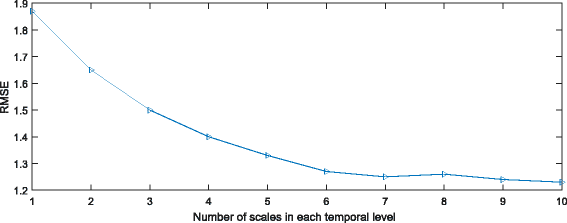

  

  RMES as a function of number of scales

  Fig. 8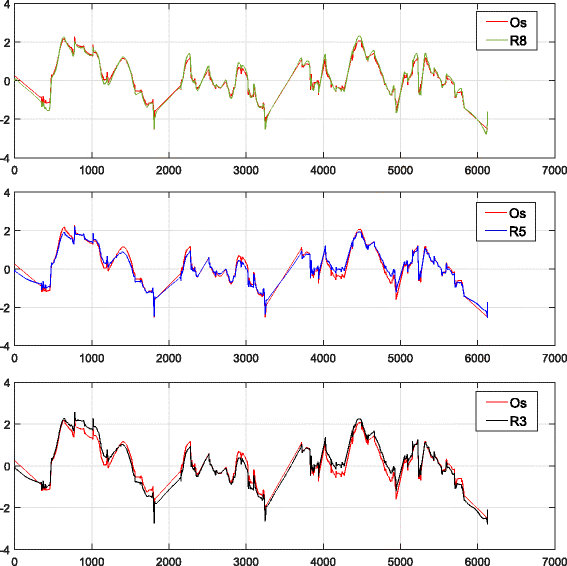

  

  Examples of original F0 signal and F0 signal reconstructed with different numbers of scales. The top graph shows the original F0 signal (Os) and the F0 signal reconstructed with eight scales in each temporal level (R8 has 8×5 scales in total); the second graph shows Os and the reconstructed signal with five scales in each temporal level (R5 has 5×5 scales in total); the bottom pan shows Os and reconstructed signal with three scales in each temporal level (R3 has 3×5 scales in total)

  where μ _src and σ _src are the mean and variance of the F0 in logarithm for the source speaker, respectively; μ _tgt and σ _tgt are the mean and variance of the F0 for target speaker, respectively; (f0 _src ) is the source speaker pitch; and (f0 _conv ) is the converted fundamental frequency for the target speaker.

• DBNs+NMF: Using the DBNs to convert spectral features while using the non-negative matrix factorization (NMF) to convert five-scale CWT-F0 features.

• DBNs+CWT(30): This is the proposed method in our previous work [21] that uses DBNs to convert spectral features while using the NNs to convert the 30-scales CWT-F0 features; each scale is separated by one third of an octave.

• DBNs+CWT(40): This method uses the same model as DBNs+CWT(30) with a different number of scales(40) in CWT-F0 features.

• DBNs+AS-CWT (proposed method): This is the proposed system that uses the DBNs to convert spectral features while using the NNs to convert the CWT-F0 features decomposed by AS-CWT method, each temporal level has eight scales (8×5 scales in total).

5.2 Objective experiment

Mel Cepstral Distortion (MCD) was used for the objective evaluation of spectral conversion, and MCD is defined below.

$$ MCD=\left(10/\ln 10 \right)\sqrt{2\sum_{i=1}^{24}\left({mc}_{i}^{t}-{mc}_{i}^{c} \right)^{2}} $$

(20)

In Eq. 20, ${mc}_{i}^{t}$ and ${mc}_{i}^{c}$ represent the target and the converted mel-cepstral, respectively.

To evaluate the F0 conversion, we used the RMSE

$$ RMSE=\sqrt{\frac{1}{N}\sum_{i=1}^{N}\left(\left(F0_{i}^{t} \right)-\left(F0_{i}^{c} \right) \right)^{2}} $$

(21)

where $F0_{i}^{t}$ and $F0_{i}^{c}$ denote the target and the converted F0 features, respectively. A lower MCD and F0-RMSE value indicate smaller distortion or predicting error. Unlike the RMSE evaluation function used in [19], which evaluated the F0 conversion by calculating logarithmic-scaled F0, we used the original target F0 and converted F0 to calculate the RMSE values. Given that our RMSE function evaluates complete sentences that contain both voiced and unvoiced F0 features instead of the voiced logarithmic scaled F0, the RMSE values are expected to be high. For emotional voices, the unvoiced features also include some emotional information. Therefore, we choose the F0 of complete sentences for evaluation instead of the voiced logarithmic scaled F0.

The average MCD and F0-RMSE results from emotional to neutral pairs are reported in Table 1. The MCD results are presented in the left part of Table 1. Comparing DBNs with source, DBNs decrease the value of MCD. As shown in Fig. 9, among DBNs+LG, DBNs+NMF, DBNs+CWT(30), DBNs+CWT(40), and DBNs+AS-CWT, MCD decreases or increases slightly, proving that the conversion of F0 does not have a significant impact on the spectral feature conversion. The F0-RMSE results are presented in the right part of Table 1. As shown in Table 1 and Fig. 10, the conventional linear conversion logarithm Gaussian can affect the conversion of happy to neutral, but only slightly affects the conversion of angry voices and sad voices to neutral voices. The NMF method, the previous CWT method, and the proposed AS-CWT method can affect the conversion of all emotional voice datasets. Comparing the results of DBN+CWT(30) and DBN+CWT(40), we see that 30 scales is the optimal number of scales for this model. Simply increasing the number of scales can not enhance the effect for DBNs+CWT. In addition, the proposed method can obtain significant improvement in F0 conversion as a whole.

Fig. 9

Mel-cepstral distortion evaluation of spectral features conversion from emotional to neutral voices

Fig. 10

Root mean-squared error evaluation of F0 features conversion from emotional to neutral voices

Table 1 MCD and F0-RMSE results for different emotions

Table 2 shows the MCD and F0-RMSE results from the neutral to emotional pairs. For spectral conversion, MCD values are deceased by the DBNs training model. However, when comparing Fig. 11 with Fig. 9, we can see that the effects of the conversion from neutral to angry and sad voices are not as significant as their inverse conversion, but the conversion from neutral to happy voice can generate better results than its inverse conversion. As shown in Fig. 12, RMSE values decrease significantly when our proposed method is used compared with other methods. When comparing Fig. 12 with Fig. 10, we can see that the CWT method and AS-CWT method can effectively convert F0 features from neutral to emotional voices and obtain better results than the conversion from emotional to neutral voices. This is because the CWT and AS-CWT models decompose the one-dimensional F0 features into several scales containing further details of different temporal scales, which modeled and captured F0 features more appropriately than the other methods as well as alleviated estimation errors. As Fig. 13 shows, the blue, red, and yellow curves represent the source, target, and converted F0, respectively. Here, we can see that after conversion using the proposed method, F0 becomes much similar to the target neutral voice.

Fig. 11

Mel-cepstral distortion evaluation of spectral features conversion from neutral to emotional voices

Fig. 12

Root mean-squared error evaluation of F0 features conversion from neutral to emotional voices

Fig. 13

Examples of source F0, target F0, and converted F0

Table 2 MCD and F0-RMSE results for different emotions

5.3 Subjective experiment

We conducted a subjective emotion evaluation via a mean opinion score test. The opinion score was set to a five-point scale (the more similar to the emotion of the sample voice the target speech sounded and the more different it is from the source speech, the larger the point given). Here, we test the emotional to neutral pairs (H2N, S2N, A2N) and their inverse conversion (N2H, N2S, N2A). In each test, 50 utterances (10 for source speech, 10 for target speech, and 30 for converted speeches using the four methods) were selected, and 10 listeners took part in the testing. Each subject listened to the source and target speech samples. Then, the subject listened to the speech converted using the four methods and was asked to give each conversion a point value. Figure 14 shows the results of the MOS test, with the error bar showing a 95% confidence interval. In this test, a higher value indicates a better result. As the figure indicates, the conventional LG method shows poor performance when converting angry voice to neutral voice. The AS-CWT method (the proposed method) obtained a better score than the LG method and NMF almost in every emotional VC t test, t>2.4, p<0.04), except for the case when converting angry voice to neutral voice (p>0.1). The difference between AS-CWT and CWT is not statistically significant when dealing with conversion from emotional voice to neutral voice and neutral voice to angry voice, because p>0.1 in the p value test, but was significant for neutral to sad (t=2.5, p=0.037) and neutral to happy (t=3.0, p=0.015).

Fig. 14

MOS evaluation of emotional voice conversion

6 Conclusions and future works

In this paper, we proposed a method using DBNs to train the MCC features to construct the mapping relationship of the spectral envelopes, while using NNs to train the CWT-F0 features. Such features are conducted by the F0 features with arbitrary scales for prosody conversion between the source and target speakers. A comparison between the proposed method and the conventional methods (logarithm Gaussian, NMF) shows that our proposed model can effectively change the acoustic and the prosody for the emotional voice at the same time.

When using this method, however, some problems remain. Specifically, the proposed model must extract the parallel speech data, which can limit the process to a one-to-one conversion only. In future works, we will explore a many-to-many emotional VC method and use it in other applications, such as emotional voice recognition [25] or facial expression recognition [26].

References

S Mori, T Moriyama, S Ozawa, in Proc. ICME. Emotional speech synthesis using subspace constraints in prosody, (2006), pp. 1093–1096.
R Aihara, T Takiguchi, Y Ariki, in Proc. SLPAT. Individuality-preserving voice conversion for articulation disorders using dictionary selective non-negative matrix factorization, (2014), pp. 29–37.
J Krivokapić, Rhythm and convergence between speakers of american and indian english. Lab. Phonol. 4(1), 39–65 (2013).
T Raitio, L Juvela, A Suni, M Vainio, P Alku, in Proc. Sixteenth Annual Conference of the International Speech Communication Association. Phase perception of the glottal excitation of vocoded speech, (2015).
Z-W Shuang, R Bakis, S Shechtman, D Chazan, Y Qin, in Proc. Ninth International Conference on Spoken Language Processing. Frequency warping based on mapping formant parameters, (2006).
D Erro, A Moreno, in Proc. Interspeech. Weighted frequency warping for voice conversion, (2007), pp. 1965–1968.
T Toda, AW Black, K Tokuda, Voice conversion based on maximum-likelihood estimation of spectral parameter trajectory. IEEE Trans. Audio Speech Lang. Process. 15(8), 2222–2235 (2007).
E Helander, T Virtanen, J Nurminen, M Gabbouj, Voice conversion using partial least squares regression. IEEE Trans. Audio Speech Lang. Process. 18(5), 912–921 (2010).
R Takashima, T Takiguchi, Y Ariki, in Proc. Spoken Language Technology Workshop (SLT). Exemplar-based voice conversion in noisy environment, (2012), pp. 313–317.
T Fukada, K Tokuda, T Kobayashi, S Imai, in Proc. ICASSP. An adaptive algorithm for mel-cepstral analysis of speech, (1992), pp. 137–140.
S Desai, EV Raghavendra, B Yegnanarayana, AW Black, K Prahallad, in Proc. ICASSP. Voice conversion using artificial neural networks, (2009), pp. 3893–3896.
T Nakashika, R Takashima, T Takiguchi, Y Ariki, in Proc. INTERSPEECH. Voice conversion in high-order eigen space using deep belief nets, (2013), pp. 369–372.
H Kawahara, Straight, exploitation of the other aspect of vocoder: perceptually isomorphic decomposition of speech sounds. Acoust. Sci. Technol. 27(6), 349–353 (2006).
K Liu, J Zhang, Y Yan, High quality voice conversion through phoneme-based linear mapping functions with straight for mandarin. Fuzzy Syst. Knowl. Discov. 4:, 410–414 (2007). IEEE.
MS Ribeiro, RA Clark, in ICASSP. A multi-level representation of f0 using the continuous wavelet transform and the discrete cosine transform (IEEE, 2015), pp. 4909–4913.
Z Luo, T Takiguchi, Y Ariki, in Proc. IEEE/ACIS 15th International Conference on Computer and Information Science (ICIS). Emotional voice conversion using deep neural networks with mcc and f0 features, (2016), pp. 1–5.
M Vainio, A Suni, D Aalto, et al, in Proc. TRASP 2013-Tools and Resources for the Analysys of Speech Prosody. Continuous wavelet transform for analysis of speech prosody, (2013).
AS Suni, D Aalto, T Raitio, P Alku, M Vainio, et al, in Proc. 8th ISCA Workshop on Speech Synthesis, Proceedings, Barcelona, August 31-September 2, 2013. Wavelets for intonation modeling in hmm speech synthesis, (2013).
H Ming, D Huang, M Dong, H Li, L Xie, S Zhang, in Affective Computing and Intelligent Interaction (ACII). Fundamental frequency modeling using wavelets for emotional voice conversion (IEEE, 2015), pp. 804–809.
H Ming, D Huang, L Xie, J Wu, M Dong, H Li, in Proc. INTERSPEECH. Deep bidirectional LSTM modeling of timbre and prosody for emotional voice conversion, (2016), pp. 2453–2457.
Z Luo, J Chen, T Nakashika, T Takiguchi, Y Ariki, in Proc. 9th ISCA Speech Synthesis Workshop. Emotional voice conversion using neural networks with different temporal scales of f0 based on wavelet transform, (2016).
T Toda, et al, Interlanguage phonology: acquisition of timing control and perceptual categorization of durational contrast in japanese (2013).
S Mallat, A wavelet tour of signal processing: the sparse way. Investigación Operacional (Academic press, Elsevier, 2008).
H Kawanami, Y Iwami, T Toda, H Saruwatari, K Shikano, GMM-based voice conversion applied to emotional speech synthesis. IEEE Trans. Speech Audio Proc, 2401–2404 (2003).
D Ververidis, C Kotropoulos, Emotional speech recognition: resources, features, and methods. Speech Comm. 48(9), 1162–1181 (2006).
J Chen, Z Luo, T Takiguchi, Y Ariki, Multithreading cascade of surf for facial expression recognition. EURASIP J. Image Video Process. 2016(1), 37 (2016).
Author information
Authors and Affiliations
Contributions
ZL designed the core methodology of the study, carried out the implementation and experiments, and he drafted the manuscript. JC participated in the study and helped to improve the proposed, he also mainly drafted the manuscript and assisted in doing experiments. TT and YA participated in the study and helped to draft the manuscript. All authors read and approved the final manuscript.
Corresponding author
Ethics declarations
Competing interests
The authors declare that they have no competing interests.
Publisher’s Note
Springer Nature remains neutral with regard to jurisdictional claims in published maps and institutional affiliations.
Rights and permissions
Open Access This article is distributed under the terms of the Creative Commons Attribution 4.0 International License(http://creativecommons.org/licenses/by/4.0/), which permits unrestricted use, distribution, and reproduction in any medium, provided you give appropriate credit to the original author(s) and the source, provide a link to the Creative Commons license, and indicate if changes were made.
About this article
Cite this article
Luo, Z., Chen, J., Takiguchi, T. et al. Emotional voice conversion using neural networks with arbitrary scales F0 based on wavelet transform. J AUDIO SPEECH MUSIC PROC. 2017, 18 (2017). https://doi.org/10.1186/s13636-017-0116-2
Received:
Accepted:
Published:
DOI: https://doi.org/10.1186/s13636-017-0116-2