From raw audio to a seamless mix: creating an automated DJ system for Drum and Bass

Abstract

We present the open-source implementation of the first fully automatic and comprehensive DJ system, able to generate seamless music mixes using songs from a given library much like a human DJ does.

The proposed system is built on top of several enhanced music information retrieval (MIR) techniques, such as for beat tracking, downbeat tracking, and structural segmentation, to obtain an understanding of the musical structure. Leveraging the understanding of the music tracks offered by these state-of-the-art MIR techniques, the proposed system surpasses existing automatic DJ systems both in accuracy and completeness. To the best of our knowledge, it is the first fully integrated solution that takes all basic DJing best practices into account, from beat and downbeat matching to identification of suitable cue points, determining a suitable cross-fade profile and compiling an interesting playlist that trades off innovation with continuity.

To make this possible, we focused on one specific sub-genre of electronic dance music, namely Drum and Bass. This allowed us to exploit genre-specific properties, resulting in a more robust performance and tailored mixing behavior.

Evaluation on a corpus of 160 Drum and Bass songs and an additional hold-out set of 220 songs shows that the used MIR algorithms can annotate 91% of the songs with fully correct annotations (tempo, beats, downbeats, and structure for cue points). On these songs, the proposed song selection process and the implemented DJing techniques enable the system to generate mixes of high quality, as confirmed by a subjective user test in which 18 Drum and Bass fans participated.

1 Introduction

When music tracks are played back to back, i.e., starting one song after the other is finished, the listening experience is interrupted between the end of a song and the beginning of the next. Indeed, popular music tracks commonly have a long intro and outro, such that the excitement of listening might fade if songs are played in full. Thus, especially for electronic dance music (EDM) in dance clubs, it is common practice for so-called disk jockeys (DJs) to blend songs together into a continuous seamless mix.

Unfortunately, DJing requires considerable expertise, specialized equipment, and time—unavailable to most music consumers. A computer program that automates the DJing task would thus democratize access to high-quality continuous music mixes outside the dance club setting. Additionally, it would alleviate the need for nightclubs and bars with a limited budget to hire expensive human DJs. Finally, professional DJs could use it as an exploration tool to discover interesting song combinations.

As DJing is a complex analytical as well as creative task, creating an automatic DJ has proved to be highly non-trivial (see Section 2). To clarify the challenges involved, next, we will discuss what a DJ is and what steps are performed to create a music mix.

1.1 What is a DJ?

A DJ is a person who mixes existing music records together in a seamless way to create a continuous stream of music [1–3]. With a seamless mix, we understand a mix that blends songs together such that the resulting music is uninterrupted (no silences in between songs), and such that the music is structurally coherent on beat, downbeat, and phrase level (see Section 3). Additionally, successive songs should be “compatible” to some extent with respect to their harmonic, rhythmic, and/or timbrical properties. In essence, a seamless mix flows from song to song such that the transition between those songs appears to be a part of the music itself, and where it consequently is often hard to tell where one song ends and the other begins. Even though there is no step-by-step “recipe” on how to DJ, there is a general consensus [1, 2] on the basic steps that the DJ executes to create a mix. As a brief introduction to the art of DJing, a simplified DJing workflow is explained below and illustrated in Fig. 1.

Fig. 1

Illustration of the simplified DJing workflow

1.1.1 Creating a mix

The DJ first selects songs to play and determines the order to play them in. This is the track selection step. The DJ selects songs that fit together thematically, rhythmically, or instrumentally, while also considering the audience’s engagement, music preference, and other factors [1–3]. There usually is a deliberate progression throughout the mix ([3], pp. 311, 328–329) for example, the DJ may start with a more relaxed song, gradually building up the energy by successively playing increasingly energetic songs. After reaching the climax, the DJ may play some calmer songs to give the crowd a rest, before building up towards a second climax, etc. The DJ also determines at what time instants in the selected songs the transition from one song into the next should start, which is called cue point selection. These starting points, or cue points, are typically aligned with structurally important boundaries in the music [1–3]: this ensures that the mix forms a contiguous piece of music that naturally “flows” from one song into another ([3], pp. 316–318).

With the songs and cue points in mind, the DJ performs the actual mixing. He or she plays the first song and waits until it reaches the cue point to start the second song. For some time, both songs will be heard simultaneously, gradually fading out the first song and fading in the next. When simultaneously playing two songs, it is imperative that their beats align in time: even a very small misalignment is easily noticed even by the amateur. To make this possible, one or both songs may have to be slowed down or sped up by time-stretching them such that their tempi are equal. The beats are then aligned in a process called beatmatching.

A smooth transition between the songs is established by performing a crossfade. This is the process of gradually increasing the volume of the new song, i.e., the fade-in, while decreasing the volume of the other song, i.e., the fade-out. The DJ also adjusts the equalization settings of the songs by adjusting the relative gain of the bass (low frequencies), mid, and treble (high frequencies): this ensures a clean sound of the mix without saturation in any of the frequency bands. Effectively, this means that the speed and profile of the crossfade may be different for different frequency bands.

The process of cueing, time-stretching, beatmatching, and crossfading is applied for each song transition, effectively creating a seamless music stream.

1.1.2 Remarks on the DJing process

It should be pointed out that the workflow described above is a simplification and not an exact step-by-step recipe of the DJing workflow. For conciseness, some aspects of the DJing process have not been elaborated on in detail. For example, depending on the audience or type of event, DJs might employ a different mixing style and consider some aspects of the process (e.g., correct beatmatching) to be less or more important than other DJs in other scenarios [2]. It should also be clear that DJing is an iterative process, i.e., the steps shown in Fig. 1 are often repeated and interwoven as the mix progresses. For example, improvisation plays an important role in DJing ([3], p. 312) and DJs do not always know beforehand which songs they will play: the track selection and cue point selection process are hence repeated “on the fly” while the DJ is mixing. For a more thorough introduction into the art of DJing, we refer to relevant works in non-academic [1, 2] and academic literature [3].

1.1.3 Understanding musical structure

It will be clear that, in order to perform the above tasks, the DJ first and foremost needs to know the tempo, beat positions, structure, and other musical properties as discussed below in Section 3.

Algorithms have been developed for each of the tasks of interest to us in this paper. However, the specific application in this paper poses specific demands on accuracy and robustness, while also offering opportunities for improvement. For example, DJing is almost invariably done with songs with a steady tempo ([3], pp. 9, 33–34) (expressed in beats per minute), making the task of tempo estimation easier than for other types of music. At the same time, the required tempo estimation accuracy exceeds the accuracy of state-of-the-art tempo estimation algorithms (see Section 5.2).

1.2 Contributions and overview

In this paper, we present a computer system that automates the tasks of a DJ. More specifically, we make the following contributions:

• The system is, to the best of the author’s knowledge, the first complete and fully integrated automatic DJ system that considers all basic DJing best practices, i.e., beatmatching, cue point selection, music style-based track selection, equalization, and different transition types. It is released as open-source¹and could hence serve as a robust basis for further research to build upon.

• The system is designed for a specific genre of electronic dance music, namely Drum and Bass. Apart from simplifying system design and dataset collection, this allows it to obtain a high structural annotation accuracy and an excellent subjective mix quality, because prior knowledge of the genre allows to exploit certain assumptions about the musical structure (see Sec. 3). For this paper, Drum and Bass was chosen given the first author’s knowledge of the genre.

• To achieve this performance, dedicated algorithms for tempo estimation, beat detection, downbeat detection, and cue point selection were developed.

• A unique feature of our proposed system is a song selection method that imitates the behavior of a professional DJ. It uses a custom style descriptor feature that projects all songs into a continuous “style space” where similar songs lie close together. This approach greatly improves the mix quality.

The remainder of this paper is structured as follows. Section 2 explores related work in scientific literature and in commercial applications. Section 3 elaborates on how the automatic DJ discovers the musical structure in a hierarchical manner. Section 4 discusses the system architecture, the song selection process, and how the song transitions are created. The system’s performance is thoroughly evaluated on different aspects in Section 5. Finally, Section 6 concludes this paper and gives some pointers for further improvements.

2 Related work

Existing research on automatic DJ systems is scarce. Two types of systems reoccur in the scientific literature: automatic DJ systems and mash-up systems (Table 1). The former attempt to automate (parts of) the DJing task, i.e., create a continuous mix by smoothly transitioning between songs. Mash-up systems on the other hand create a new song by combining short fragments of existing songs. A mash-up is typically much shorter than a DJ mix, and the input songs are more heavily modified by cutting and pasting fragments from them. Nevertheless, similar techniques, such as time-stretching, beat tracking, and crossfading, are used in both applications.

Table 1 Overview of existing (automatic) DJ software and related work

Jehan [4] proposes a simple automatic DJ system that automatically matches downbeats and crossfades songs. Cue points are determined by finding rhythmically similar sections in the mixed songs, but it does not consider the high-level structure of the music. Bouckenhove and Martens [5] describe a system that uses vocal activity detection to avoid overlapping vocal sections of two songs. With their Music Paste system, Lin et al. [6] automate the track and cue point selection process by maximizing a measure for musical similarity. The length of the transition is optimized such that the rate of tempo change remains under an acceptable threshold, which is determined in a subjective experiment. Ishizaki et al. [7] also focus on the optimization of a crossfade with a changing tempo. They propose to use an intermediary tempo in between the tempi of the original songs, such that the discomfort caused by the tempo change is spread evenly between the two songs. Finally, the MusicMixer project by Hirai [8] improves the track and cue point selection process by means of two similarity measures related to the beat structure and a high-level abstraction of the chromatic content of the audio, inspired by natural language processing techniques.

Research on mash-up systems typically focuses on devising a measure of musical compatibility of song extracts. An example is the AutoMashUpper system by Davies et al. [9, 10], which features a beat tracking, downbeat tracking, and a structural segmentation step to align the music. Music fragments are extracted based on their harmonic and rhythmic similarity. Lee et al. [11] focus on extending mash-up systems to multiple overlapping songs and also consider the compatibility of consecutive music segments instead of only the compatibility of the overlapped segments.

Most existing work on automatic DJ systems focuses on optimizing individual crossfades by minimizing the amount of discomfort. However, there are still some important limitations to these systems. First of all, the crossfading process often remains very simple, e.g., without performing any equalization. Secondly, very few systems consider the high-level structural properties of the mixed audio. Thirdly, the focus is usually on optimizing individual crossfades, but the global song progression throughout the mix is not considered. In general, there appears to be no complete integrated DJing system in scientific literature that elegantly combines all necessary components and considers DJing best practices to create enjoyable music mixes.

There also exist many commercial DJing applications. Examples of professional DJing software include Serato DJ [12] and Traktor Pro 2 [13] or free alternatives such as VirtualDJ [14] and Mixxx [15, 16]. These aid the DJ in analyzing the music by annotating, e.g., the tempo, beat and downbeat positions, and the musical key. Most of this software is tailored to DJs who perform the mixing themselves using advanced DJing equipment such as turntables and mixers, but some feature automatic DJing functionality as well. Another application designed for DJs is Mixed In Key [17], which aids DJs in performing harmonic mixing. It is not DJing software itself, but rather an annotation tool that extracts a song’s key, tempo, relevant cue points, and a custom “energy-level” annotation. Mixed In Key can be integrated with DJing software such as Serato DJ or Traktor Pro 2. The company behind Mixed In Key also released Mashup2, a mashup creation program that features automatic beat matching and key compatibility detection [18]. There also exist apps whose main purpose is to automate the task of a DJ. Examples include the mobile apps Serato Pyro [19] and Pacemaker [20]. However, the automatic DJ capabilities in commercial applications remain quite simple. Typically, the transitions follow a basic “intro-outro” paradigm, where the next song is played only when the current song ends [21, 22]. Informal experimentation furthermore indicates an inferior performance in terms of beat detection accuracy and no or only very basic cue point selection capabilities. Finally, none of the aforementioned commercial applications are open-source or explain the inner workings of their algorithms. Hence, to the best of our knowledge, no well-documented, open-source automatic DJ solution exists that combines existing MIR knowledge and DJing best practices as in the proposed project.

A common trend in existing work is to deal with a broad variety of genres. However, the presented system is designed to explicitly deal with only one genre, namely Drum and Bass. In their One In The Jungle paper, Hockman, Davies, and Fujinaga [23] already point out the need for genre-specific approaches within MIR research, more specifically for genres like Drum and Bass that have for example very distinct drum patterns. The proposed system gives further proof that a genre-specific approach might indeed be beneficial for certain applications.

3 Discovering the musical structure

One characteristic of music as an audio signal is that it exhibits a hierarchical structure [3, 24]. At the lowest level, music consists of individual musical events or notes, which repeat periodically to define the tempo of the music. Certain events (typically percussive in nature) are more prominent than others, creating the beats. In Drum and Bass, like in most types of EDM, beats can be grouped into groups of four ([3], pp. 246–248), which are called measures or bars. The first beat of a measure is called the downbeat of that measure. Measures are the basic building blocks of longer musical structures such as phrases, which then make up the larger sections that determine the compositional layout of the song. The typical composition of a Drum and Bass song is illustrated in Fig. 2.

Fig. 2

Example of the compositional layout of a Drum and Bass song ([3], pp.287–292). A song typically starts with an intro, followed by a build-up that gradually increases the musical tension. This tension is released in a moment called the drop, which is the beginning of the main section or core ([3], p. 289) of the music, comparable to the chorus in pop music. After the main section, there is a musical bridge, also called a breakdown, that connects the first main section and the second build-up, drop, and main section. An outro gradually brings the music to a close. Note that this structure is not fixed and that many variations are of course possible

Knowing the rhythmical and structural properties of the music is extremely important for a DJ. The tempo and beat positions are used to beatmatch the music. The high-level musical structure is important when selecting cue points: if the DJ mixes songs where the downbeats or segment boundaries are not appropriately aligned, the mix will most likely sound structurally incoherent ([3], pp. 317–318).

The automatic DJ system is designed for a specific music genre, and it therefore makes several assumptions about the music’s structural properties:

• The music’s tempo is between 160 and 190 beats per minute and is assumed to be constant throughout the song,

• The music has a strict 4/4 time signature, i.e., there are four beats to a bar,

• Phrases are a multiple of 8 measures long, and musical segments are an integer number of phrases long. Boundaries between segments are accentuated by large changes in musical texture.

Even though these assumptions might seem restrictive, they are based on extensive experience with the target music genre and should hold for a vast majority of Drum and Bass songs. Some of these properties have also been noted in other works for EDM in general ([3], pp. 246–248). Furthermore, we believe that it is feasible to adapt the mentioned techniques to different EDM genres (see Section 6).

In what follows is described how the proposed DJ system extracts the beat, downbeat, and segment boundary locations from the audio in a hierarchical way given the assumptions listed above.

3.1 Beat tracking

To discover the beat positions, an algorithm inspired by the work of Davies and Plumbley [25] is used. It assumes a constant tempo, which is the case for the vast majority of Drum and Bass music. With this assumption, only two parameters need to be determined to define the positions of all the beats: the beat period τ (expressed in seconds) or equivalently the tempo $\nu =\frac {60}{\tau }$ (expressed as “beats per minute”), and the beat phase ϕ (expressed in seconds), i.e., the time difference between the first beat and the start of the audio signal. Two observations are at the core of the beat tracking algorithm. Firstly, most repetitions of musical onsets, e.g., played notes or percussion events, happen after an integer number of beats. Secondly, the loudest or most prominent onsets typically occur on beat locations. To exploit these observations, the positions of musical onsets are estimated by means of an onset detection function (ODF), which has a high value for time instants in the music where an onset is detected, and a low value elsewhere. An excellent review on the different types of onset detection functions is given by Bello et al. [26].

Figure 3 illustrates the beat tracking algorithm. The first step is to calculate the ODF Γ(m) of the audio. The melflux ODF is used [27] with a frame size N_F of 1024 samples and hop size N_H of 512 samples. The audio sample rate f_s is 44100 Hz. With the notations explained in Table 2, X_mel40(m,k) being the energy of frame m in the k^th frequency bin, logarithmically spaced according to the Mel scale [28], and HWR the half-wave rectify operation HWR(x)=max(x,0), the ODF is calculated as follows:

$$ \Gamma(m) = \sum\limits_{k=1}^{40}\text{HWR}(X_{\text{mel40}}(m,k) - X_{\text{mel40}}(m-1,k)). $$

(1)

Fig. 3

Illustration of the beat tracking algorithm. a Audio waveform extract. b Half-wave rectified onset detection function Γ_HWR(m). c Autocorrelation function A_Γ(l) of the ODF. d Tempo detection curve $\mathcal {B}(\tau)$. e Phase detection curve Φ(ϕ). Our algorithm’s estimate of the beat period $\hat {\tau }$ and the beat phase $\hat {\phi }$ are annotated. This figure was created by applying the algorithm to a piece of audio of 4 m 30 s long. For illustrative purposes, only the first few seconds of the audio waveform, ODF and autocorrelation function are shown. Note that the described algorithm detects the beats between 160 and 190 BPM, and a larger tempo range is shown in d for illustrative purposes

Table 2 Overview of mathematical notations used in this paper

This curve is post-processed by subtracting a running mean with window size Q frames from it and half-wave rectifying the result:

$$\begin{array}{*{20}l} \bar{\Gamma}(m) &= \underset{m - \frac{Q}{2} \leq q \leq m + \frac{Q}{2}}{\text{mean}}\left\{\Gamma(q)\right\} \text{,} \end{array} $$

(2)

$$\begin{array}{*{20}l} {\Gamma}_{\text{HWR}}(m) &= \text{HWR}\left(\Gamma(m) - \bar{\Gamma}(m)\right)\text{.} \end{array} $$

(3)

Q is set to 16 ODF frames, as in [25]. Then, the beat period is extracted by calculating the autocorrelation function A_Γ(l) of the ODF:

$$A_{\Gamma}(l) =\frac{1}{M}\sum_{m}{\Gamma_{\text{HWR}}(m)\Gamma_{\text{HWR}}(l+m)}. $$

(4)

The autocorrelation A_Γ(l) is large at lag values l that are a multiple of the beat period τ. Thus, we propose to estimate the beat period τ as the one for which the sum of autocorrelation values at corresponding lags (integer multiples of τ) is maximal. Concretely, we define the tempo detection curve$\mathcal {B}(\tau)$ as:

$$ \mathcal{B}(\tau) = \frac{1}{N}\sum_{n}{} A(n\,L_{\tau}), $$

(5)

and obtain an estimate $\hat \tau$ for the beat period as:

$$ \hat{\tau} = \underset{\tau}{\text{argmax}}(\mathcal{B}(\tau)), $$

(6)

with a corresponding lag value $L_{\hat {\tau }}$ (in frames). Note that $L_{\hat {\tau }}$ does not need to be an integer. The beat phase is determined by summing the ODF values for every possible time shift ϕ between 0 and $\hat {\tau }$, at fixed intervals of one beat period. The phase is then estimated as the one leading to the highest sum. Formally, defining the phase detection curve as:

$$ {\Phi}(\phi)= \frac{1}{N}\sum_{n} \Gamma_{\text{HWR}}(n \,L_{\hat{\tau}} + L_{\phi}), $$

(7)

the phase is estimated as:

$$ \hat{\phi} = \underset{\phi}{\text{argmax}}({\Phi}(\phi)). $$

(8)

The estimated position of the m’th beat is (with ⌊·⌉ rounding to the nearest integer):

$$\begin{array}{*{20}l} t_{\text{beat}}^{(m)} &= m \hat{\tau} +\hat{\phi} &\text{(in seconds)}, \end{array} $$

(9)

$$\begin{array}{*{20}l} L_{\text{beat}}^{(m)} &= \lfloor m L_{\hat{\tau}} + L_{\hat{\phi}} \rceil &\text{(in frames)}, \end{array} $$

(10)

$$\begin{array}{*{20}l} N_{\text{beat}}^{(m)} &= \lfloor m N_{\hat{\tau}} + N_{\hat{\phi}} \rceil &\text{(in samples)}. \end{array} $$

(11)

The tempo range is restricted between 160 BPM and 190 BPM (160≤ν≤190), because the tempo of Drum and Bass music falls between these values. We consider increments of 0.01 BPM for the tempo and 1 ms for the phase.

3.2 Downbeat tracking

Given the beat positions, the proposed DJ system determines which beats are downbeats. Since measures of 4 beats long are assumed, there are only four options: the first downbeat of the song is either the first, the second, the third or the fourth beat, and every fourth beat after that beat is also a downbeat. The downbeat tracking algorithm is summarized in Fig. 4. It consists of three main steps. First, features are extracted from the beat segments. Then, a logistic regression classifier, trained on 117 manually annotated songs, determines the probability that a beat is either the first, second, third, or fourth beat in measure it belongs to. Finally, these predictions are aggregated over the entire song for each of the four options to determine the most likely downbeat positions.

Fig. 4

Overview of the downbeat tracking algorithm. a The audio waveform, annotated with beats and downbeats. b Isolated features are extracted from the beats. c Isolated features are combined to create contextual features. d The machine learning model classifies each beat, estimating the log-probability of a beat being either the 1st, 2nd, 3rd, or 4th beat in a measure. e The downbeats are determined by summing the log-probabilities along each possible trajectory and choosing the most likely one. Here, the second trajectory is highlighted

For features, the loudness [29] of each beat fragment and the energy distribution of the audio along the frequency axis, binned in 12 equally spaced bins on the Mel frequency scale [28], are calculated. Additionally, three onset detection functions are calculated of the entire song, namely the flux, the high-frequency coefficient (HFC), and the complex spectral difference (CSD) ODF. Different ODFs capture different musical onset events [26], and informal experimentation indicated that using multiple ODFs greatly improves performance. With the notations from Table 2, this gives:

$$\begin{array}{*{20}l} x_{\text{frame}}^{[N_{\hat{\tau}};N_{\hat{\tau}}]}(m) &= x[{N_{\hat{\tau}}(m)}:{N_{\hat{\tau}}(m+1)}], \end{array} $$

(12)

$$\begin{array}{*{20}l} \mathcal{X}_{\text{loud}}(m) &= \text{loudness}\left(x_{\text{frame}}^{[N_{\hat{\tau}};N_{\hat{\tau}}]}(m)\right), \end{array} $$

(13)

$$\begin{array}{*{20}l} \mathcal{X}_{\text{mel}}(m,k) &= X_{\text{mel12}}\left(x_{\text{frame}}^{[N_{\hat{\tau}};N_{\hat{\tau}}]}(m)\right)(k), \end{array} $$

(14)

$$\begin{array}{*{20}l} \mathcal{X}_{\text{odf}_{i}}(m,k) &= \Gamma_{\text{HWR}}^{\text{(i)}}(L_{\text{beat}}^{(m)} + k),\, 0 \leq k < L_{\hat{\tau}},i \in\\& \{\text{flux}, \text{csd}, \text{hfc}\}. \end{array} $$

(15)

The features are standardized by subtracting the mean and dividing by the standard deviation of the corresponding features in all beats of the song. These features describe each beat in isolation and are therefore called isolated features. However, a beat fragment does not contain enough information on its own to determine its position within its measure. Indeed, the notion of rhythmical structure arises by the carefully orchestrated accentuation of certain beats compared to other beats. Therefore, the proposed machine learning classifier uses so-called contextual features$\mathcal {X}^{\text {ctxt}}$ that describe differences between the isolated features of a given beat and those of the next 4 or 8 beats. For the different types of isolated features, they are calculated as follows, with m the current beat index, k the subfeature index if the isolated feature is a vector, l the lag in number of beats with which the isolated feature vector is compared, and i∈{flux,csd,hfc}:

$$ \mathcal{X}_{\text{loud}}^{\text{ctxt}}(m,l) = \mathcal{X}_{\text{loud}}(m+l) - \mathcal{X}_{\text{loud}}(m), 0 < l < 8, $$

(16)

$$ {\begin{aligned} \mathcal{X}_{\text{mel}}^{\text{ctxt}}(m,l,k) \,=\, \mathcal{X}_{\text{mel}}(m\,+\,l,k) \,-\, \mathcal{X}_{\text{mel}}(m,k), & l \in \{-1,1,2,3\}, \end{aligned}} $$

(17)

$$ {\begin{aligned} \mathcal{X}_{\text{odf,corr}}^{\text{ctxt,(i)}}(m,l) &= \sum\limits_{k=0}^{L_{\hat{\tau}}-1}{\Gamma^{\text{(i)}}(L_{beat}^{(m+l)}+ k) \Gamma^{\text{(i)}}(L_{beat}^{(m)} + k) }, & \\&\qquad\qquad\qquad\qquad\qquad l \in \{-1,1,2,3\}, \end{aligned}} $$

(18)

$$ {\begin{aligned} \mathcal{X}_{\text{odf,int}}^{\text{ctxt,(i)}}(m,l) &=\sum\limits_{k=0}^{L_{\hat{\tau}}-1}\Gamma^{\text{(i)}}(L_{beat}^{(m+l)} + k) & \\ &-\sum\limits_{k=0}^{L_{\hat{\tau}}-1}{\Gamma^{\text{(i)}}((L_{beat}^{(m)} + k)}, & 0 < l < 16. \end{aligned}} $$

(19)

Initial experimentation indicated that the downbeat machine learning model is much less reliable in the less “expressive” parts of the audio, e.g., the intro and the outro. Therefore, beats in the intro and outro are trimmed away using a heuristic iterative algorithm based on the RMS energy of the beats. Figure 5 shows this algorithm in pseudo-code. First, the RMS value of every beat’s audio is calculated. This sequence of RMS values is smoothed using a running mean operation, and then the first and last beat in the audio are determined where the running mean RMS value is larger than a threshold, i.e., a fraction of the maximum running mean RMS value. If more than 40% of all beats lie in between these boundaries, those beats are kept to determine the downbeats. Else, the threshold is decremented and the algorithm is repeated until at least 40% of the beats are “selected.” The threshold fraction is initialized at 0.9 and is decremented in steps of 0.1.

Fig. 5

Pseudo-code for the audio trimming algorithm of the downbeat tracker

To determine the downbeats of a song, the algorithm works as follows (see Fig. 4). First, the audio is trimmed using the aforementioned algorithm. Then, the features of the remaining beats are extracted and subsequently classified using the machine learning model. This results in a log-probability vector for each beat that estimates whether it is either the first, second, third or fourth beat in its measure. The algorithm then exploits the assumption that the music has a strict 4/4 time signature: for each of the four possible trajectories throughout the song, the corresponding log-probabilities of the beats are summed, and the trajectory with the highest sum is the most likely and is predicted to be correct. Finally, this prediction is extrapolated to the trimmed beats in the intro and outro, after which all downbeat positions are known.

3.3 Structural segmentation

The high-level compositional structure of the song is discovered using the novelty-based structural segmentation method by Foote [30]. This approach assumes that structural boundaries are accompanied by significant musical changes in the audio. It uses a so-called structural similarity matrix (SSM) S(m,n), which generally is constructed by splitting the input audio into short frames, extracting features of those frames and comparing the features of each frame with those of every other frame, resulting in a matrix of pairwise comparisons. The automatic DJ system uses not one, but two SSMs, both using an analysis frame length of half a beat long ($N_{\hat {\tau }} / 2$ samples) and a hop size of a quarter beat ($N_{\hat {\tau }} / 4$ samples). As features, one SSM uses 13 MFCCs per measure, and the other uses the frames their RMS energy. The distance between the MFCC feature vectors is calculated using the cosine distance; for the RMS features, the absolute scalar difference is used:

$$ d_{\text{cos}}(n{u},\vec{v}) = 1 - \frac{\vec{u} \cdot \vec{v}}{\|\vec{u}\|_{2} \|\vec{v}\|_{2}}, $$

(20)

$$ {\begin{aligned} {X}_{\text{MFCC}}^{[N_{\hat{\tau}}/2;N_{\hat{\tau}}/4]}(m,k) = X_{\text{MFCC}}\left(x_{\text{frame}}^{[N_{\hat{\tau}}/2;N_{\hat{\tau}}/4]}(m)\right)(k), \end{aligned}} $$

(21)

$$ {\begin{aligned} S_{\text{MFCC}}(m,n) = d_{\text{cos}}\left(X_{\text{MFCC}}^{[N_{\hat{\tau}}/2;N_{\hat{\tau}}/4]}(m,\cdot), X_{\text{MFCC}}^{[N_{\hat{\tau}}/2;N_{\hat{\tau}}/4]}(n,\cdot)\right), \end{aligned}} $$

(22)

$$ \mathcal{X}_{\text{RMS}}^{[N_{\hat{\tau}}/2;N_{\hat{\tau}}/4]}(m) = \sqrt{\text{mean}\left\{\left(x_{\text{frame}}^{[N_{\hat{\tau}}/2;N_{\hat{\tau}}/4]}(m)\right)^{2} \right\}}, $$

(23)

$$ S_{\text{RMS}}(m,n) = \left|\mathcal{X}_{\text{RMS}}^{[N_{\hat{\tau}}/2;N_{\hat{\tau}}/4]}(m)- \mathcal{X}_{\text{RMS}}^{[N_{\hat{\tau}}/2;N_{\hat{\tau}}/4]}(n)\right|. $$

(24)

Similar frames lead to a low value in the matrix, whereas dissimilar frames result in high values (Fig. 6a). The formation of blocks in the matrix indicates the occurrence of musically coherent segments. The algorithm by Foote determines the location of the boundaries between these segments by convolving the matrix along its main diagonal with a “checkerboard” kernel $\mathcal {K}$:

$$\begin{array}{*{20}l} {\mathcal{K}}(k,l) = \left\{\begin{array}{ll} 1& {\text{for}}\ kl \geq 0,\\ -1& {\text{for}}\ kl < 0. \end{array}\right. \end{array} $$

(25)

Fig. 6

Illustration of structural segmentation concepts. a Example of a structural similarity matrix. The audio waveform is shown next to both axes. b Calculation of the novelty curve by convolving the SSM with a checkerboard kernel along the diagonal

This leads to a novelty curve Γ^(SSM,i)(m), which has high values for time instants at a structural boundary and low values elsewhere (with i∈{RMS,MFCC}, and K the kernel width in frames):

$$\begin{array}{*{20}l} \Gamma^{\text{(SSM,i)}}(m) = \left|\sum\limits_{k=-\frac{K}{2}}^{\frac{K}{2}} \sum\limits_{l=-\frac{K}{2}}^{\frac{K}{2}} \mathcal{K}(k,l) S_{i}(m+k,m+l)\right|. \end{array} $$

(26)

K is equal to 64 frames, i.e., 4 measures before and after each time instant are used to determine the novelty at that instant. This process is illustrated in Fig. 6b. Finally, both novelty curves are combined by taking the element-wise geometric mean of both curves:

$$ \Gamma^{\text{(SSM)}}(m) = \sqrt{ \Gamma^{\text{(SSM,RMS)}}(m) \Gamma^{\text{(SSM,MFCC)}}(m)}. $$

(27)

The geometric mean will only show a peak when both curves have a peak at the same time. Hence, the geometric mean gives the novelty curve for boundaries on which both individual curves “agree.” This operation is based on the observation that boundaries between segments often go along with changes in harmonic content and musical texture as well as changes in musical energy ([3], pp. 290–292, 297–298), which the MFCC SSM and RMS SSM respectively attempt to capture.

Given the audio’s novelty curve, phrase-aligned structural segment boundaries are determined. Figure 7 summarizes this process in pseudo-code. Structural boundaries are extracted by first selecting the 20 highest peaks in the novelty curve. Several post-processing steps based on musically inspired rules are applied to determine the downbeat-aligned boundary positions. First, the peaks positions, which—given the SSM time resolution—are detected at a half-beat granularity and hence could initially be at non-downbeat positions, are rounded to the nearest downbeat. Peaks that lie further than 0.4 times the length of a measure from a downbeat are discarded as false positives. From the downbeat-aligned segment boundary candidates, a subset is determined in which all candidates lie at a multiple of 8 measures from each other, because phrases are assumed to be 8 measures long. In what follows, candidate boundary positions are denoted p_i (in downbeats) and their amplitudes are denoted a_i. For each subset, all peak amplitudes are summed that do not occur one or two measures before another peak with a novelty value greater than 0.75 times the amplitude of the peak considered for summation. This reduces the number of false positives caused by breaks, i.e., short musical segments that break up the music and typically occur just before a structural boundary. Each sum is multiplied by the number of peaks contributing to it, increasing the importance of a sum with many contributors. The structural boundary candidates that contributed to the highest sum are considered to be the correct boundaries.

Fig. 7

Pseudo-code for selecting phrase-aligned boundaries given the SSM novelty curve in the structural segmentation algorithm

Each segment is then assigned a label based on its RMS energy: segments with an average RMS energy higher than the average song-wide RMS energy get a label “high,” whereas quieter segments get a label “low.” This labeling method attempts to tag the “main” or “core” sections of the song with a label “high” and the other sections (intro, buildup, breakdown, …) as “low.” This is used to determine cue points, as described in Section 4.2.3.

4 Composing a DJ mix

Section 3 described how the proposed DJ system analyzes music to gain a detailed understanding of it much like a human DJ has. The current section elucidates how the proposed DJ system also simulates parts of the creative process of a human DJ, i.e., a creative track and cue point selection and a variation of transition types, leveraging the detailed musical understanding to generate high-quality mixes.

4.1 Automatic DJ system architecture

The automatic DJ system architecture is shown in Fig. 8. Songs are annotated offline using the beat tracker, downbeat tracker and structural segmentation modules. Additionally, the replay gain [31] is annotated, which allows to play all songs at an equal volume, regardless of the volume they were recorded at. Also the key (Section 4.2.1), style descriptor (Section 4.2.2) and the beat tracking ODF are determined.

Fig. 8

Automatic DJ system architecture. On the left, in yellow, are the annotation submodules. On the right, in green, are the modules used “live” during the mixing process

The mix generation and playback happen “live” by iteratively performing track and cue point selection, time-stretching, beatmatching, and crossfading, as detailed below.

During the mixing process, the track and cue point selection algorithm determines the next song and cue points, given the current song. Three transition types, inspired by how professional DJs compose their mix and perform crossfades, are possible. The type is chosen using a Finite State Machine, which ensures variation in the mix by preventing that certain transition types happen twice in a row. The transition type defines which segments (“low” or “high”) of the first song and the new song are overlapped, i.e., it defines possible cue points (Section 4.2.3). The next song is selected such that the resulting mix is musically coherent as a whole while ensuring that individual song transitions are enjoyable to listen to. Details of this selection process are explained in Section 4.2.

Once the cue points are known, the crossfade is established. This happens by time-stretching the audio, applying volume fading and equalization filters and then adding the two songs together in a beatmatched way. The tempo is fixed at 175 BPM for the entire mix. This process is explained in more detail in Section 4.3.

4.2 Track and cue point selection

The track and cue point selection is done in five steps that iteratively narrow down the options for potential successors of the current song. Firstly, only songs that are in key with the current song are considered (Section 4.2.1). Of these songs, the six most similar songs in terms of musical style are selected as potential successors (Section 4.2.2). In the third step, cue points are determined for the current song and for the candidate successors (Section 4.2.3). The two final steps heuristically estimate the musical quality of each potential overlap. More specifically, vocal activity is detected such that overlapping vocals of both songs is avoided (Section 4.2.4), and rhythmic similarity is estimated by comparing the songs their ODFs (Section 4.2.5). The song with the highest rhythmic similarity to the current song and without vocal clashes is selected as the next song.

4.2.1 Musical key compatibility

Mixing in key or harmonic mixing is a technique often employed by professional DJs where successive songs have the same or a related key [1, 2]. This ensures that they fit together harmonically and reduces dissonance when playing two songs at the same time. Even though recent work [32] questions the use of harmonic mixing based on the musical key in specific cases, e.g., for music outside the major/minor scale framework, to the best of our knowledge, the technique is still common practice in Drum and Bass. Hence, the automatic DJ system features a simple key extraction implementation.

The key of each song is discovered in a pre-processing step using the algorithm by Faraldo et al. [33], which is implemented in the Essentia music analysis library [34] and has been tuned to electronic dance music in particular. The annotations are stored on disk, allowing fast retrieval. The allowed key changes for the next song are going a perfect fifth up or down (i.e., changing to the dominant or subdominant key) or changing to the relative key of the key of the current song. Only the songs that are in one of these keys or in the same key as the current song are considered in the following steps. This choice of allowed keys is inspired by DJing best practices [1, 17] and they are related to the music theory concept of the circle of fifths. This is illustrated in Fig. 9 [24].

Fig. 9

Illustration of the circle of fifths and allowed key changes in the DJ system. For example, if the key of the current song is C major (light gray), the allowed key changes are one perfect fifth up (G major, the dominant key), one perfect fifth down (F major, the subdominant key) or changing to the relative key (A minor)

To give the automatic DJ more song options to choose from, also the songs in a key one semitone lower or higher than one of the related keys are added to the pool. If one of these would eventually be selected as the next song, its key will be altered using a process called pitch shifting. This involves subsequently time-stretching and then down- or upsampling the audio, effectively changing the music’s pitch without altering the playback speed. This is necessary since a key one semitone below or above a compatible key is usually not a compatible key itself.

4.2.2 Musical style descriptor

A DJ often mixes songs that are similar in style, genre, or atmosphere. In what follows, the term style describes the combination of timbre, mood and energy of a song. For example, a song might be energetic or calm in nature, uplifting or moody, happy or dark and so on. The automatic DJ describes the style by means of a custom style descriptor feature.

Two much-cited approaches of content-based audio similarity measures are those by Logan [35] and by Aucouturier [36]. The former models the distribution of frame-wise spectral features by means of a K-means cluster model, whereas the latter constructs a Gaussian mixture model of the feature vectors. Song similarity is calculated using respectively the Earth Mover Distance algorithm and a sampling approach. However, these approaches are computationally expensive, both to construct the song models as for evaluating the distance metrics [37].

To limit the annotation and song comparison time, the automatic DJ adopts a simpler approach. First, spectral contrast features [38, 39] are extracted from short overlapping frames of audio, using a frame size and hop size of respectively 2048 and 1024 samples. Only the audio belonging to “high” segments from the structural segmentation task are used, as these typically make up the most recognizable and descriptive parts of the music ([3], p. 290). The spectral contrast features calculate the ratio between the magnitudes of peaks and valleys within different sub-bands of the spectrum and in this way describe the relative amount of harmonic and noise components in those bands. They reportedly outperform MFCC features for music genre classification [39], as confirmed by informal experiments. Of these frame-wise features, the means and variances of the individual vector components are calculated across all frames, and also the mean and variances of the first-order differences, resulting in a 48-dimensional vector describing each audio file:

$$ \mathcal{X}_{\text{contrast}}^{[2048;1024]}(m,k) = \text{spectral-contrast}\left(x_{\text{frame}}^{[2048;1024]}(m)\right), $$

(28)

$$ \mathcal{X}_{\text{style,mean}}(k) = \underset{m}{\text{mean}}\left(\mathcal{X}_{\text{contrast}}^{[2048;1024]}(m,k)\right), $$

(29)

$$ \mathcal{X}_{\text{style,stdev}}(k) = \underset{m}{\text{stdev}}\left(\mathcal{X}_{\text{contrast}}^{[2048;1024]}(m,k)\right), $$

(30)

$$ {{} \begin{aligned} \mathcal{X}_{\text{style,\(\Delta\),mean}}(k) &= \underset{m}{\text{mean}}\left(\mathcal{X}_{\text{contrast}}^{[2048;1024]}(m,k)\right.\\&\quad \left.-\mathcal{X}_{\text{contrast}}^{[2048;1024]}(m-1,k)\right), \end{aligned}} $$

(31)

$$ {{} \begin{aligned} \mathcal{X}_{\text{style,\(\Delta\),stdev}}(k)& = \underset{m}{\text{stdev}}\left(\mathcal{X}_{\text{contrast}}^{[2048;1024]}(m,k)\right.\\&\quad\left.-\mathcal{X}_{\text{contrast}}^{[2048;1024]}(m-1,k)\right),\\ \end{aligned}} $$

(32)

$$ {{} \begin{aligned} \mathcal{X}_{\text{style}} = \left[\mathcal{X}_{\text{style,mean}}, \mathcal{X}_{\text{style,stdev}}, \mathcal{X}_{\text{style,\(\Delta\),mean}}, \mathcal{X}_{\text{style,\(\Delta\),stdev}}\right]. \end{aligned}} $$

(33)

The vector $\mathcal {X}_{\text {style}}$ is then projected onto a lower-dimensional feature space in which thematically similar songs lie close together and dissimilar songs are further apart. This projection is done by projecting them onto the top three dimensions found by applying principal component analysis (PCA) on a collection of 160 Drum and Bass songs. The resulting three-dimensional representation will be called the style descriptor$\Theta = \text {PCA}_{3}(\mathcal {X}_{\text {style}})$. The Euclidean distance between two style descriptors measures song similarity.

Before describing how the DJ system’s track selection algorithm uses the style descriptor, an analysis of the behavior of the style descriptor in professional DJ mixes is presented to motivate our approach. In this analysis, several professional mixes downloaded from the internet were analyzed by extracting 90 s of music with a hop size of 120 s. These parameters were chosen after informally determining the average duration of an individual song in a DJ mix. The evolution of the style descriptor throughout three professional DJ mixes is visualized in Fig. 10a–c. The style stays in a relatively small neighborhood compared to the entire collection of songs in the music library. Therefore, to imitate this behavior, the automatic DJ system should also select songs that stay relatively close to one another (Fig. 10d). Note that this observation also strengthens the hypothesis that the style descriptor groups thematically similar songs close together, since professional DJs typically select quite similar songs for a mix [3, 317–320].

Fig. 10

Illustration of the style descriptor progression throughout six DJ mixes. The gray dots represent the style descriptors of 513 Drum and Bass songs, selected from different sub-genres of Drum and Bass. The black dots mark the songs in the mix. Successive songs are connected by a line. a, b, c Professional DJ mixes, resp. [54–56]. d, e, f Generated DJ mixes. The style centroid is marked by a red dot. d Default settings for (α,β)=(0.4,− 0.1). e Large β: (α,β)=(0.4,− 0.9). f No style centroid, large β: (α,β)=(0,− 0.5)

The song selection process works as follows. Before the mix is started, the automatic DJ randomly selects the first song and selects the quarter of all the songs in the music library that are closest to this first song in the style descriptor space. The centroid of the style descriptors of these songs will be called the style centroid Θ_centroid. During generation, the DJ calculates the ideal style of the next song $\hat {\Theta }_{next}$ as a weighted sum of the current song’s descriptor, the previous song’s descriptor, and the style centroid. With α and β the weight of the style centroid and of the previous song respectively, this gives:

$$ {\hat{\Theta}}_{next}= \alpha\,{\Theta}_{centroid} + (1-\alpha)\left(\beta\,{\Theta}_{prev} + (1-\beta)\,{\Theta}_{cur}\right). $$

(34)

α and β have been arbitrarily assigned the values 0.4 and − 0.1 respectively. The centroid weight α ensures that all songs stay relatively close to the style centroid, leading to a thematically uniform mix. A value of α close to 1 will keep the mix centered around the style centroid, while a value close to 0 allows the mix to “wander” freely through the style space, leading to a more varied but potentially less uniform mix (Fig. 10f). A negative weight for β is chosen such that there is a deliberate progression or “flow” of the style: the next song will be dissimilar to the current song in a similar way as the current song is dissimilar to the previous song. A more negative β leads to larger the jumps in style between successive songs (Fig. 10e), again presenting a trade-off between variation and coherence. Figure 10d illustrates the default behavior of the automatic DJ system, while Fig. 10e, f shows the effect of alternative settings for α and β.

The pool of song candidates is reduced by only keeping the songs that are closest to ${\hat {\Theta }}_{next}$. In the current prototype of the automatic DJ, six songs are kept.

4.2.3 Cue point selection

To determine cue points, the automatic DJ first chooses one out of three transition types. These types differ in what types of structural segments are overlapped (“high” or “low” energy) and hence determine the allowed cue point positions. For the different transition types, this selection happens as follows (as illustrated in Fig. 11):

• Double drop: in both the current and the next song, the cue points are chosen 16 measures before a drop, i.e., a transition from a low to a high segment. In the current song, the first drop after the current playback instant is used; in the next song, if there are multiple drops, then one is picked at random. The fade-in and fade-out are 16 and 32 measures long respectively. The drops of both songs are aligned in time, hence the name double drop.

  Fig. 11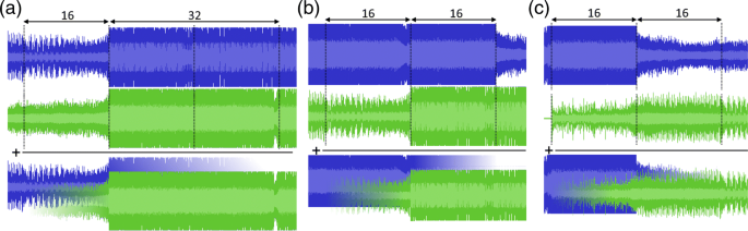

  

  Illustration of the cue point selection for the three transition types. The fade-in and fade-out lengths, expressed in number of measures, are annotated. Also the final crossfades are conceptually illustrated. a Double drop. b Rolling transition. c Relaxed transition

• Rolling transition: the cue point in the current song is 32 measures before the next transition from a high to a low segment. The cue point in the next song is the downbeat 16 measures before a drop. The fade-in and fade-out are both 16 measures long. In this transition, the second song its drop continues the energetic nature of the high section of the preceding song.

• Relaxed transition: the cue point in the current song is 16 measures before the next transition from a high to a low segment. The next song is started at the beginning, i.e., its first structural boundary. The fade-in and fade-out are both 16 measures long. In this way, the energetic nature of the mix is interrupted, giving the listener some time to relax.

The transition type is chosen pseudo-randomly by means of a finite state machine that specifies the probability of selecting each type, given the previous transition’s type (Table 3). The current implementation balances a rather high-energy “flow” (high probabilities for rolling transitions) with moments to rest (relaxed transitions) and exciting climaxes (double drops). To avoid layering too many songs at once, double drops are not allowed after a rolling transition or another double drop.

Table 3 Transition matrix controlling the transition type selection

After determining the transition type, cue points are determined for each of the six remaining song candidates. Given that particular choice of cue points, the automatic DJ system estimates the quality of the crossfades in the two final steps to make a final selection for the next song.

4.2.4 Vocal clash detection

When two songs are mixed together, it is important to avoid vocal clashes as this might disrupt the listening experience, especially when the vocals have a predominant presence in both songs ([3], p. 318). Even though Drum and Bass is a predominantly instrumental genre, vocals regularly occur. For this reason, a vocal activity detection mechanism is built into the automatic DJ system.

Existing work on singing voice detection [40–42] typically adopts a machine learning approach, where features extracted from short frames of audio are classified as either vocal or instrumental. The output is then smoothed using for example an HMM or ARMA filtering [42, 43]. Unfortunately, at the time of implementing the DJ system, no software implementation of a vocal activity detection solution was available that could be easily integrated into the automatic DJ system. A simple baseline solution is developed instead. A support vector machine classifier with an RBF kernel is trained to classify segments of one measure long. The segments are first analyzed in frames of 2048 samples long with a halve frame overlap between consecutive frames. Of these short frames, 13 MFCCs, 6 spectral contrast, and the corresponding 6 spectral valley features [39] are calculated. The means, variances, and skews of these features are calculated, as well as the means and variances of the first-order differences of features in consecutive frames, giving 250 features for each downbeat segment. These are the input to the SVM classifier. The training set consists out of 55 manually annotated songs. The classifier parameters were tuned using cross-validation, giving a regularization parameter C of 1.0 and kernel coefficient γ of 0.01. During the annotation process, the SVM classification of each measure is stored on disk to be used in the song selection process.

The classification output is post-processed before using it for song selection. A measure is labeled “vocal” if either the measure itself or both its neighboring measures are classified as “vocal” by the SVM: else the measure gets the label “instrumental.” A vocal clash is detected if at least two “vocal” measures overlap; a one-measure overlap is tolerated. Only the songs and cue points are considered that do not lead to a vocal clash. If however all candidates lead to a clash, the clash is tolerated for that transition.

4.2.5 Onset detection function matching

Rhythmic similarity is estimated by comparing the songs their onset detection functions. The ODFs from the beat tracking process are stored on disk and are used for this comparison. The ODF portions corresponding to the overlapped music segments are compared by means of the dynamic time warping (DTW) algorithm, since the ODFs are calculated for the audio at their original (unstretched) tempo. The DTW algorithm stretches the ODFs during comparison and hence eliminates the need to recalculate the ODFs after time-stretching the original audio. A second motivation for the DTW algorithm is that small rounding errors occur when selecting an extract from the ODFs, as beat positions often do not align with an ODF frame boundary. Because of this, two ODF extracts that are very alike might be shifted one or two frames with respect to each other: therefore, some flexibility is allowed. However, a beam search strategy is applied to prevent excessive warping of the compared ODFs. The song and cue point combination which leads to the lowest DTW score is selected as optimal.

4.3 Creating the crossfade

Given the next song and the cue point positions, the crossfade is established. Time-stretching is performed by applying harmonic-percussive separation [44] and independently stretching the harmonic and percussive residuals, respectively using the frequency-domain phase vocoder [45] and the time-domain OLA time scale modification algorithm [46], as proposed by Driedger and Müller [47]. This approach significantly reduces audio artifacts compared to traditional time-stretching algorithms at the expense of a higher computational cost [48]. Afterwards, volume fading and equalization filters are applied to both songs. The exact crossfade patterns for each transition type were manually defined to ensure a smooth transition between songs. During the fade-in, the volume of the next song gradually rises to full level, while its bass and treble remain almost entirely filtered out. At the end of the fade-in, a switch occurs between the songs: the bass and treble of the next song are quickly increased to full level, and at the same time the bass and treble of the previous song are filtered out. The volume of the previous song is then gradually faded out until the end of the crossfade. This particular equalization pattern ensures that the bass and treble of only one song will be heard at any point during the crossfade, leading to a clean, unsaturated sound of the resulting mix. Finally, the audio of the songs is added together in a beatmatched fashion, effectively mixing the two songs together.

5 Results and discussion

The automatic DJ system has been tested on different aspects. First, the system’s execution time is measured and the envisaged setup is described. Then, the accuracy of the different annotation methods from Section 3 is evaluated. Additionally, the vocal activity detection algorithm is evaluated on its ability to discriminate between clashing and non-clashing crossfades. Finally, a subjective user test assesses the efficacy of the style descriptor and the ODF matching and tests the system as a whole. These evaluations have been performed using three sets of songs: a first set of 117 songs (Additional file 2 Table S1), a second set of 43 songs (Additional file 2 Table S2), and a third set of 220 songs (Additional file 2 Table S3). When referring to the set of 160 songs, the combination of the first and second set is meant. A full tracklisting of all three sets has been provided in an additional file.

5.1 System performance and envisaged setup

The presented DJ system mixes “live”, i.e., it generates future transitions in the background while the music is playing. On a consumer-grade laptop (4-thread Intel Core i7-6500U CPU at 2.50 GHz, 8 GB RAM), it takes 17.0 s on average to generate the next transition (averaged over 100 generated transitions; standard deviation 6.6 s, maximum 32.2 s). This is less than 16 measures of music at 175 BPM (≈22 s). In the current implementation, two consecutive transitions start at least 16 measures (and typically more) apart from each other, ensuring that the system does not hang because it is waiting for the next transition to be generated. Furthermore, a buffer mechanism queues multiple transitions as an additional safeguard that prevents the system from running out of music.

The annotation of the input music library happens offline, i.e., before the actual mixing process can start. Annotating one song takes 12.0 s on average, i.e., 2.3 s per minute of audio on average (standard deviation 0.1 s; evaluated on 160 songs). As a coarse guideline, we recommend at least 50 to 100 Drum and Bass songs in the input music library in order to create a 30-min mix (≈ 20 transitions) of good quality. Of course, the more songs in the library, the more flexibility the automatic DJ has, and the better the mix will be.

5.2 Evaluation of the beat tracker

The beat tracking accuracy is evaluated on a collection of 160 Drum and Bass songs. The annotations made by the beat tracker are not compared with a manually annotated ground truth, because this manual labeling is extremely time consuming and because the inherent ambiguity of the beat annotation task [49] makes this even more difficult. Instead, the annotation correctness is evaluated by overlaying the audio with beep sounds at the beat positions detected by the algorithm and listening if they coincide with the true beat positions in the music. To avoid listening to the entire song, two 15-s fragments are evaluated per song: one a quarter into the song, and one three quarters into the song. If a fragment is beatless (e.g., because at that moment in the song there happens to be a breakdown), a new fragment with beats is chosen near that position and is evaluated instead. Large beat tracking errors, such as a large tempo error (e.g., 1 BPM or more) or a wrong phase, are clearly audible when listening to only one of the fragments. The second fragment is used to detect small tempo errors: even if in the first fragment the beat positions appear to be correct, they are unlikely to be correct in the second fragment because the tempo deviation would cause the beat annotations to “drift away” from the correct beat positions. Among different candidates, the melflux ODF, as implemented in the Essentia library [34], performs best with 159 out of 160 songs annotated correctly, i.e., an accuracy of 99.4%. A second evaluation on a second test set of 220 songs leads to an accuracy of 98.2%, i.e., four songs their beats are incorrectly detected. In these cases, the tempo is still detected correctly, but the phase is wrong by half a beat period, such that the detected beat positions lie exactly in between the correct beats.

To motivate the need for a custom beat tracker, this paragraph discusses the behavior of existing beat tracker implementations. Experiments with several open-source implementations [34, 50] show that these annotate beat positions that are often not exactly equidistant, either because the algorithms are tailored towards songs with a variable tempo or because the specific implementation is not entirely accurate. We illustrate this in more detail for the BeatDetectionProcessor beat tracker from the madmom music processing library [50] on the first and second set of songs (resp. 160 and 220 songs). Even though the madmom documentation claims it detects beats at a constant tempo, slight inter-beat interval (IBI) variations occur: on average, the IBI standard deviation within a song is 2.2% of the correct IBI length. This happens because it detects the IBI as an integer number of ODF frames, even though the IBI usually is a non-integer number of frames long, and then fixes rounding errors by detecting beats using a tolerance interval. Using these non-equidistant beat positions would complicate for example the beat matching implementation, and a constant IBI throughout the entire song is much more desirable. However, averaging the IBIs leads to significant tempo estimation errors ($\hat {\nu }=\frac {60}{mean_{i}(IBI_{i})}$): for 115 out of 380 tested songs (30.3%), the estimation differs more than 0.25 BPM from the real tempo, and for 59 songs (15.5%), the error is even higher than 0.5 BPM. This is considered too inaccurate for an automatic DJ system, explaining the need for a custom beat tracker that uses an exact, constant IBI between all beats.

5.3 Evaluation of the downbeat tracker

The downbeat tracking machine learning model has been trained on a training set of 117 annotated songs, and its performance is evaluated on a hold-out test set of 43 songs. The ground-truth downbeat position is annotated as a single label per song (1, 2, 3, or 4), which denotes whether the first beat of the song, and every fourth beat after that, is either the 1^st, 2^nd, 3^rd or 4^th beat in the measure it belongs to. This of course assumes that the beat positions are annotated: these annotations are created using the algorithm described in Section 3.1 and manually determining the tempo and phase of the songs where the beat tracker made a mistake. On individual beat segments, i.e., by taking the argmax for each per-beat log-probability prediction (step (d) in Fig. 4) and before summing the log-probabilities (so before step (e) in Fig. 4), the downbeat classifier achieves an accuracy of 75.4% (excluding beats in the intro and outro). On a song level, i.e., after summing the log-probability vectors of the individual beats and predicting a single song-wide downbeat index, the downbeat tracker achieves an accuracy of 95.3% on the 43 test songs. On the second test set of 220 songs, four of the 214 songs with correct beat annotations had incorrect downbeat annotations, leading to an accuracy of 98.1%.

The need for a custom downbeat tracker is motivated mainly because existing downbeat trackers implemented in open-source libraries were found to be less accurate on this corpus of music and additionally require more computation time. We evaluated this in more detail by running the RNNBarProcessor downbeat tracker from the madmom library [50] on 160 songs, given the ground-truth beat annotations as input. The algorithm takes 35.4 s per song on average (standard deviation 6.7 s) to calculate the downbeat positions, compared to 4.47 s (standard deviation 1.4 s) for the DJ system’s implementation. Furthermore, 20 songs their downbeat position were wrong, which gives an accuracy that is considerably worse than the presented downbeat tracker (87.5% compared to 98.1%).

5.4 Evaluation of the structural segmentation task

The accuracy of the structural segmentation task is more difficult to assess because of its subjective nature [51]. Here, annotations are considered structurally correct if they belong to the correct subset of downbeats at a multiple of eight measures from each other (see Section 3.3). Additionally, the simple labeling of the segments as a “low” or a “high” segment is evaluated. To do so, every transition from a “low” to a “high” segment in each of the 160 songs is listened to and is considered correct if that transition coincides with a drop in the music (see Fig. 2). For 3 out of 160 songs, the 8-measure offset was incorrect. For 4 out of 160 songs, the assumption that all segmentation boundaries lie at a multiple of 8 measures from each other is incorrect. This means that 95.3% of the songs received structurally correct annotations. For 82.4% of these songs, also the drop detection as a “low” to a “high” transition is correct. In the second test set, 94.3% of the songs with correct downbeat annotations also received structurally correct segmentation annotations.

5.5 Evaluation of the song filtering

The SVM classifier for vocal activity detection has been trained on a manually annotated selection of 55 songs, containing 12,260 downbeat segments in total of which 2321 contain vocal activity. Data augmentation is performed by pitch shifting the audio for training one semitone up and down, artificially tripling the amount of training data. The unequal class sizes are countered by choosing class weights inversely proportional to the class size [52]. The classifier achieves an accuracy, precision, recall and F1-score of respectively 97.8%, 90.2, 99.2, and 94.5% on the train set and 87.0, 62.3, 61.1, and 61.7% on a hold-out test set of 38 manually annotated songs containing 8524 downbeats (7097 non-vocal and 1427 vocal downbeats), where the vocal label is considered to be the positive class.

The ability to detect vocal clashes in transitions is evaluated by calculating all overlaps between all pairs of manually annotated songs that would be possible in the automatic DJ system. Each overlap is assigned a label clashing if vocals overlap in at least two measures in the resulting mix (as in the DJ system, an overlap of one measure is tolerated). The same label is estimated using the singing voice detection model. The confusion matrix for this experiment is shown in Table 4. This shows that about 69.3% of the vocal clashes can be prevented, at the expense of falsely discarding 16.5% of the non-clashing crossfades.

Table 4 Confusion matrix for the vocal clash detection experiment (No clash: 10167 crossfades; Clash: 1524 crossfades)

5.6 User study: evaluation of the musical style descriptor and system evaluation

Figure 10 informally validates the ability of the style descriptor feature to group similar songs close together and separate dissimilar songs. To provide a more robust evaluation, a subjective user test has been carried out.

Two mixes are generated using an input library of 380 songs. One mix has all automatic DJ functionality enabled, in the other the songs are selected without considering the style descriptor. The mixes are both 15 min long and contain 10 and 11 transitions respectively. Both only use songs with structurally correct annotations, to ensure that any loss in mix quality is the result of the track selection process and not of an annotation error. Additionally, both mixes start with the same song. Eighteen Drum and Bass fans were asked to listen to both mixes and select which mix had the best track selection in their opinion. These fans were reached through online Drum and Bass fora; they were not paid to take part in the experiment. The users are told that both the mixes are generated by the DJ system. They also rated each mix with a score from 1 to 5, where 5 is the best possible score. Histograms of these ratings are shown in Fig. 12. In the same user test, two other mixes are presented to the users using a similar procedure to evaluate the ODF matching procedure. In the first mix, all automatic DJ functionality is enabled, and in the second, the ODF matching is reversed such that the worst matching song is selected instead of the best match. The ratings for both mixes are compared in Fig. 12. The user test results are shown in Table 5.

Fig. 12

User test results: comparison of the ratings by the users. a Style descriptor track selection vs. style-agnostic track selection. b Automatic DJ vs. song selection of worst matching songs in terms of ODF overlap

Table 5 User test results

This test indicates that the style descriptor selection process drastically improves the mix consistency and its perceived quality, with 17 out of 18 evaluators preferring that mix (p value 7.25×10⁻⁵). Figure 12a also shows that the mix with the style descriptor received higher ratings on average (an average rating of 3.89 versus 2.39 respectively). The ODF matching mix was also preferred more often than the reversed matching scenario, but the distinction is less clear (10 out of 15 evaluators², p value 0.151, and an average rating of 3.76 versus 3.41 respectively). The user tests also resulted in valuable qualitative feedback³. The first mix with all DJ features was received very well. Compared to the second mix (style-agnostic track selection), it was said to be “more consistent,”“tunes that match in style and feel,” that it had “more continuity” and less dissonance. The mix with style-agnostic track selection was critiqued as being “too rushed,” changing too much between sub-genres and that it “sounded like a DJ that was occasionally just throwing tunes into the mix without much thought.” Only one user preferred the second mix over the first, because “it incorporates more vocals, this makes me think that it is more likely to be made by a human.” The transition quality for the second set of mixes was more or less the same according to many participants, which indicates that selecting songs based on ODF similarity might not significantly influence the mix quality. Nevertheless, as there is a slight preference towards the ODF-based selection, this feature is kept in the DJ system. Other informal feedback indicates that the key detection algorithm and the vocal activity detection might need improvement, as some users noticed bad harmonic mixing or vocal clashes in some transitions.

6 Conclusions

The automatic DJ system presented in this paper generates a seamless music mix from a library of Drum and Bass songs. It uses beat tracking, downbeat tracking and structural segmentation algorithms to analyze the structural properties of the music. Evaluated on a hold-out test set of 220 songs, a beat tracking accuracy of 98.2%, a downbeat tracking accuracy of 98.1% and a segmentation accuracy of 94.3% is achieved, meaning that in total 90.9% of the songs get structurally correct annotations. This efficacy is made possible in part by adopting a genre-specific approach. The extracted structural knowledge is used in a rule-based framework, inspired by DJing best practices, to create transitions between songs. To the best of the authors’ knowledge, this system is the first that combines all basic DJing best practices in one integrated solution. Musical consistency between songs is ensured by employing a harmonic mixing technique and a custom style descriptor feature. The track selection algorithm also optimizes the rhythmic onset pattern similarity in the overlapped music segments and avoids vocal clashes by means of a support vector machine classifier. A subjective evaluation in which 18 Drum and Bass fans participated indicates that the style descriptor feature for song selection drastically improves the mix quality. The influence of the ODF similarity matching is less clear. Overall, the automatic DJ system is able to seamlessly join together Drum and Bass songs and create an enjoyable mix.

However, some aspects of the system could still be evaluated in more detail, while others could be improved or extended. An obvious direction of further evaluation is to adapt the proposed system to different EDM genres. For some genres, this can be as straightforward as adapting the tempo range, and potentially retraining the downbeat tracker on some annotated songs in the target genre. However, as different genres might require different styles of mixing [2], for some genres, more modifications might be required (e.g., implementing additional transition types). Additionally, comparing the different transition types or even the DJ system as a whole with for example transitions performed by a human expert or a commercial automatic DJ system would also be very informative, and offers a great direction of further research. Several extensions and augmentations are also possible. Firstly, the annotation modules would benefit from a built-in reliability measure to discard songs with uncertain annotations. Furthermore, the used vocal activity detection and key estimation algorithms are simple baseline versions and subject to improvement. To improve the cue point selection, a finer distinction between section types could be implemented, instead of only considering “low” and “high” sections. This could lead to more precise cue point positions or a more diverse set of transition types. It would furthermore be very interesting to make the volume and equalization progressions throughout the transitions adapt to the songs being mixed, instead of following a fixed pattern as in the current implementation. Finally, even though the track selection method yields pleasing results, it might be an oversimplification of how professional DJs compose their sets and create a deliberate progression of energy and mood throughout the mix. A model that better understands the long-term structures and composition of a good Drum and Bass mix, e.g., learned using the abundance of professional Drum and Bass mixes that can be found online, might therefore lead to a better result.

To conclude, we highlight the potential of an automatic DJing system, e.g., integration in audio streaming services to create an infinite DJ mix from a huge collection of music, as an assisting tool for human DJs to quickly explore their music libraries, or even as a substitute for a human DJ. Allowing the human DJ or the audience to interact with the automatic DJ system is also a very intriguing direction of future work, as this could lead to many new creative applications that were previously not possible. This automated approach is furthermore not constrained by the limitations of a human: it can mix together an arbitrary number of songs with fine-grained control over the equalizer settings, explore a myriad of song combinations before choosing the optimal one, and modify or even generate music on the fly. It remains an open question whether a computer could eventually become equally good or even better than professional DJs. After all, what characterizes good DJs is a certain performance element, their strong connection with the crowd, their deep insight in the music and their ability to consistently surprise in so many creative ways—aspects that are challenging to automate. Nevertheless, automated DJ systems have a great creative potential, and open up many interesting options for both listeners and DJs.

References

J. Steventon, DJing for dummies (Wiley, New Jersey, 2014).
F. Broughton, B. Brewster, How to DJ (properly) - the art and science of playing records (Bantam Press, London, 2006).
M. J. Butler, Unlocking the groove: rhythm, meter, and musical design in electronic dance music (Indiana University Press, Bloomington, 2006).
T. Jehan, Creating music by listening. PhD thesis, Massachusetts Institute of Technology (2005).
D. Bouckenhove, J. Martens, Automatisch Mixen Van Muzieknummers Op Basis Van Tempo, Zang, Energie En Akkoordinformatie, Ghent University (2007). https://lib.ugent.be/catalog/rug01:001312437.
H. -Y. Lin, Y. -T. Lin, M. -C. Tien, J. -L. Wu, in Proceedings of the 10th International Society for Music Information Retrieval Conference. Music paste: concatenating music clips based on chroma and rhythm features (ISMIRKobe, 2009), pp. 213–218.
H. Ishizaki, K. Hoashi, Y. Takishima, in Proceedings of the 10th International Society for Music Information Retrieval Conference. Full-automatic DJ mixing system with optimal tempo adjustment based on measurement function of user discomfort (ISMIRKobe, 2009), pp. 135–140.
T. Hirai, in Proceedings of the 12th International Conference on Advances in Computer Entertainment Technology. MusicMixer : computer-aided DJ system based on an automatic song mixing (ACEIskandar, 2015).
M. E. P. Davies, P. Hamel, K. Yoshii, M. Goto, in Proceedings of the 14th International Society for Music Information Retrieval Conference. AutoMashUpper: an automatic multi-song mashup system (ISMIRCuritiba, 2013), pp. 575–580.
M. E. P. Davies, P. Hamel, K. Yoshii, M. Goto, AutoMashUpper: automatic creation of multi-song music mashups. IEEE/ACM Trans. Speech Lang. Process. (TASLP). 22(12), 1726–1737 (2014). https://doi.org/10.1109/TASLP.2014.2347135.
C. l. Lee, Y. T. Lin, Z. R. Yao, F. Y. Lee, in Proceedings of the 16th International Society for Music Information Retrieval Conference. automatic mashup creation by considering both vertical and horizontal mashabilities (ISMIRMálaga, 2015), pp. 399–405.
Serato, Serato DJ software (2017). https://serato.com/dj. Accessed 15 May 2017.
Native Instruments GmbH, Traktor Pro 2 (2017). https://www.native-instruments.com/en/products/traktor/dj-software/. Accessed 15 May 2017.
Atomix Productions, Virtual DJ (2017). https://www.virtualdj.com/. Accessed 15 May 2017.
Mixxx, Mixxx (2017). https://www.mixxx.org/. Accessed 15 May 2017.
T. H. Andersen, in CHI’05 Extended Abstracts on Human Factors in Computing Systems. In the Mixxx: novel digital DJ interfaces (ACMNew York, 2005), pp. 1136–1137. https://doi.org/10.1145/1056808.1056850.
M. I. K. LLC, Mixed In Key software (2018). https://mixedinkey.com/. Accessed 06 July 2018.
M.I.K. LLC, Mashup2 software (2018). https://mixedinkey.com/. Accessed 06 July 2018.
Serato, Serato Pyro (2017). https://seratopyro.com/. Accessed 15 May 2017.
Pacemaker Music AB, Pacemaker (2017). https://pacemaker.net/. Accessed 15 May 2017.
D. White, Casual DJ Mixing Apps in Pacemaker + Spotify: should DJs be worried? (2015). https://djtechtools.com/2015/12/17/casual-dj-mixing-app-spotify-and-pacemaker/. Accessed 05 Sept 2017.
D. White, Serato Pyro: Can A Casual App Take Over House Party DJing? (2016). http://djtechtools.com/2016/02/11/serato-pyro-can-a-casual-app-take-over-house-party-djing/. Accessed 05 Sept 2017.
J. Hockman, M. Davies, I. Fujinaga, in Proceedings of the 13th International Society for Music Information Retrieval Conference. One in the jungle: downbeat detection in hardcore, jungle, and Drum and Bass (ISMIRPorto, 2012), pp. 169–174.
M. Pilhofer, H. Day, Music theory for dummies (Wiley, New Jersey, 2015).
M. E. P. Davies, M. D. Plumbley, Context-dependent beat tracking of musical audio. IEEE Trans. Audio, Speech Lang. Process.15(3), 1009–1020 (2007). https://doi.org/10.1109/TASL.2006.885257.
J. P. Bello, L. Daudet, S. Abdallah, C. Duxbury, M. Davies, M. B. Sandler, A Tutorial on onset detection in music signals. IEEE Trans. Audio, Speech Lang. Process.13(5), 1035–1047 (2005).
D. P. W. Ellis, Beat Tracking by dynamic programming. J. N. Music. Res.36(1), 51–60 (2007). https://doi.org/10.1080/09298210701653344.
S. S. Stevens, J. Volkmann, E. B. Newman, A scale for the measurement of the psychological magnitude pitch. J. Acoust. Soc. Am.8(3), 185–190 (1937).
S. S. Stevens, The measurement of loudness level. J. Acoust. Soc. Am.27(5), 815–829 (1955). https://doi.org/10.1121/1.1912650.
J. Foote, Automatic audio segmentation using a measure of audio novelty. Int. Conf. Multimed. Expo. 1(C), 452–455 (2000). https://doi.org/10.1109/ICME.2000.869637.
D. Robinson, ReplayGain specification (2014). http://wiki.hydrogenaud.io/index.php?title=ReplayGain_specification. Accessed 15 May 2017.
R. B. Gebhardt, J. Margraf, in 13th International Symposium on Computer Music Multidisciplinary Research (CMMR). Applying psychoacoustics to key detection and root note extraction in edm, (2017).
Á. Faraldo, E. Gómez, S. Jordà, P. Herrera, in Advances in Information Retrieval - 38th European Conference on IR Research, ECIR 2016, Padua, Italy. Key estimation in electronic dance music (SpringerCham, 2016), pp. 335–347.
D. Bogdanov, N. Wack, E. Gómez, S. Gulati, P. Herrera, O. Mayor, G. Roma, J. Salamon, J. R. Zapata, X. Serra, in Proceedings of the 14th International Society for Music Information Retrieval Conference. Essentia: an audio analysis library for music information retrieval (ISMIRCuritiba, 2013), pp. 493–498.
B. Logan, A. Salomon, A music similarity function based on signal analysis, in IEEE International Conference on Multimedia and Expo, ICME, (2001), pp. 22–25.
J. -J. Aucouturier, F. Pachet, et al., in 3rd International Conference on Music Information Retrieval (ISMIR), Paris, France. Music similarity measures: What’s the use? (2002), pp. 13–17.
E. Pampalk, S. Dixon, G. Widmer, in Proceedings of the sixth international conference on digital audio effects (DAFx-03), London. On the evaluation of perceptual similarity measures for music, (2003), pp. 7–12.
D. -N. Jiang, L. Lu, H. -J. Zhang, J. -H. Tao, L. -H. Cai, in Proceedings. IEEE International Conference on Multimedia and Expo, 1. Music type classification by spectral contrast feature, (2002), pp. 113–116. https://doi.org/10.1109/ICME.2002.1035731.
V. Akkermans, J. Serrà, P. Herrera, in Proceedings of the Sound and Music Computing Conference (SMC), Porto, Portugal. Shape-based spectral contrast descriptor, (2009), pp. 143–148.
A. L. Berenzweig, D. P. Ellis, in Proceedings of the 2001 IEEE Workshop on the Applications of Signal Processing to Audio and Acoustics. Locating singing voice segments within music signals (IEEENew Platz, 2001), pp. 119–122.
S. Leglaive, R. Hennequin, R. Badeau, in 2015 IEEE International Conference on Acoustics, Speech and Signal Processing (ICASSP). Singing voice detection with deep recurrent neural networks (IEEEBrisbane, 2015), pp. 121–125.
H. Lukashevich, M. Gruhne, C. Dittmar, Effective singing voice detection in popular music using arma filtering (Workshop on Digital Audio Effects (DAFx’07), Bordeaux, 2007).
M. Ramona, G. Richard, B. David, in 2008 IEEE International Conference on Acoustics, Speech and Signal Processing. Vocal detection in music with support vector machines (IEEELas Vegas, 2008), pp. 1885–1888.
D. Fitzgerald, Harmonic/percussive separation using median filtering (13th International Conference on Digital Audio Effects (DAFX10), Graz, 2010).
J. L. Flanagan, R. Golden, Phase vocoder. Bell Lab. Tech. J.45(9), 1493–1509 (1966).
W. Verhelst, M. Roelands, An overlap-add technique based on waveform similarity (WSOLA) for high quality time-scale modification of speech. IEEE Int. Conf. Acoust., Speech, Signal Process.2(1), 2–5 (1993). https://doi.org/10.1109/ICASSP.1993.319366.
J. Driedger, M. Muller, S. Ewert, Improving time-scale modification of music signals using harmonic-percussive separation. IEEE Signal Process. Lett.21(1), 105–109 (2014).
J. Driedger, M. Müller, A review of time-scale modification of music signals. Appl. Sci.6(2), 57 (2016).
M. Müller, Fundamentals of music processing: audio, analysis, algorithms, applications (Springer. https://doi.org/10.1007/978-3-319-21945-5.
S. Böck, F. Korzeniowski, J. Schlüter, F. Krebs, G. Widmer, in Proceedings of the 24th ACM International Conference on Multimedia. madmom: a new python audio and music signal processing libraryAmsterdam, The Netherlands, 2016), pp. 1174–1178. https://doi.org/10.1145/2964284.2973795.
J. Paulus, M. Müller, A. Klapuri, in Proceedings of the 11th International Society for Music Information Retrieval Conference. Audio-based music structure analysis (ISMIRUtrecht, 2010), pp. 625–636.
C. -C. Chang, C. -J. Lin, Libsvm: a library for support vector machines. ACM Trans. Intell. Syst. Tech. (TIST). 2(3), 27 (2011).
L. Vande Veire, Supplementary material: results of user test (2017). https://docs.google.com/spreadsheets/d/e/2PACX-1vRpvbHqnvlwpG9qBlaHBth3_FNmu7HeD0Ycp6ePFQ7sN_COhBOQ9pfMt4eu5lwgHp1aQAPSMrI7lPUD/pubhtml. Accessed 05 Sept 2017.
Optical, FABRICLIVE Promo Mix (2014). https://soundcloud.com/fabric/optical-fabriclivepromomix. Accessed 15 May 2017.
S.P.Y, FABRICLIVE x Back To Basics Mix (2014). https://soundcloud.com/fabric/spy-fabriclive-x-back-to-basics-mix. Accessed 31 July 2018.
Bass Brothers, FABRICLIVE x Playaz Mix (2014). https://soundcloud.com/fabric/bassbrothers-fabriclive-x-playaz-mix. Accessed 31 July 2018.
Acknowledgements
We are grateful to Paolo Simeone for insightful discussions over the course of the research reported on in this paper. The research leading to these results has received funding from the European Research Council under the European Union’s Seventh Framework Programme (FP7/2007-2013)/ERC Grant Agreement No. 615517, and from the FWO (project no. G091017N, G0F9816N).
Author information
Authors and Affiliations
Contributions
LVV developed the methods and software, conducted all experiments and the user study, and wrote most of the paper. TDB conceived the project, provided advise throughout the project, advised on the structure of the paper, and edited the text. Both authors read and approved the final manuscript.
Corresponding author
Ethics declarations
Competing interests
The authors declare that they have no competing interests.
Publisher’s Note
Springer Nature remains neutral with regard to jurisdictional claims in published maps and institutional affiliations.
Additional information
Availability of data and materials
All code is made available as open-source and can be downloaded from https://bitbucket.org/ghentdatascience/dj under an AGPLv3 license.
Authors’ information
Len Vande Veire is currently a PhD Fellow of the Research Foundation of Flanders (FWO) at Ghent University - imec, IDLab, Department of Electronics and Information Systems. Most of the research described in this paper was conducted during his Master’s thesis and a summer internship at the research group of prof. De Bie. Tijl De Bie is full professor at Ghent University, IDLab, Department of Electronics and Information Systems.
Additional file
Additional file 1
Table S1: Tracklist of the training set (117 songs). Table S2: Tracklist of the test set (43 songs). Table S3: Tracklist of the additional test set (220 songs). (PDF 35 kb)
Rights and permissions
Open Access This article is distributed under the terms of the Creative Commons Attribution 4.0 International License (http://creativecommons.org/licenses/by/4.0/), which permits unrestricted use, distribution, and reproduction in any medium, provided you give appropriate credit to the original author(s) and the source, provide a link to the Creative Commons license, and indicate if changes were made.
About this article
Cite this article
Vande Veire, L., De Bie, T. From raw audio to a seamless mix: creating an automated DJ system for Drum and Bass. J AUDIO SPEECH MUSIC PROC. 2018, 13 (2018). https://doi.org/10.1186/s13636-018-0134-8
Received:
Accepted:
Published:
DOI: https://doi.org/10.1186/s13636-018-0134-8