- Research
- Open access
- Published:
Loudness stability of binaural sound with spherical harmonic representation of sparse head-related transfer functions
EURASIP Journal on Audio, Speech, and Music Processing volume 2019, Article number: 5 (2019)
Abstract
In response to renewed interest in virtual and augmented reality, the need for high-quality spatial audio systems has emerged. The reproduction of immersive and realistic virtual sound requires high resolution individualized head-related transfer function (HRTF) sets. In order to acquire an individualized HRTF, a large number of spatial measurements are needed. However, such a measurement process requires expensive and specialized equipment, which motivates the use of sparsely measured HRTFs. Previous studies have demonstrated that spherical harmonics (SH) can be used to reconstruct the HRTFs from a relatively small number of spatial samples, but reducing the number of samples may produce spatial aliasing error. Furthermore, by measuring the HRTF on a sparse grid the SH representation will be order-limited, leading to constrained spatial resolution. In this paper, the effect of sparse measurement grids on the reproduced binaural signal is studied by analyzing both aliasing and truncation errors. The expected effect of these errors on the perceived loudness stability of the virtual sound source is studied theoretically, as well as perceptually by an experimental investigation. Results indicate a substantial effect of truncation error on the loudness stability, while the added aliasing seems to significantly reduce this effect.
1 Introduction
Binaural technology aims to reproduce 3D auditory scenes with a high level of realism by endowing the auditory display with spatial hearing information [1, 2]. With the increased popularity of virtual reality and the advent of head-mounted displays with low-latency head tracking [3], the need has emerged for methods of audio recording, processing, and reproduction, that support high-quality spatial audio. Spatial audio gives the listener the sensation that sound is reproduced in 3D space, leading to immersive virtual soundscapes.
A key component of spatial audio is the head-related transfer function (HRTF) [4]. An HRTF is a filter that describes how listener’s head, ears, and torso affect the acoustic path from sound sources arriving from all directions into the ear canal [5]. An HRTF is typically measured for an individual in an anechoic chamber using an HRTF measurement system [6–8]. Alternatively, a generic HRTF is measured using a manikin. Prior studies have shown that personalized HRTF sets yield substantially better performance in both localization and externalization of a sound source, compared to a generic HRTF [9, 10].
A typical HRTF is composed from signals from several hundreds to thousands of directions measured on a sphere around a listener, using a procedure which requires expensive and specialized equipment and can take a long time to complete. This motivates the development of methods that require fewer spatial samples, but still enable the estimation of HRTF sets at high spatial resolution. Although advanced signal processing techniques can reduce the measurement time [11], specialized equipment is still needed. Together with reducing the measurement time, methods with fewer samples may be devised with relatively simple measurement systems. For example, while a system for measuring an HRTF with hundreds of measurement points may require a loudspeaker system with expensive mechanical scanning [12], and when many fewer samples are required, the scanning system could be abandoned, and one loudspeaker could be placed at each desired direction, leading to a simpler and more affordable system. In addition, a small number of spatial samples may be efficacious in real-time applications, which require computational efficiency for real-time implementation [13, 14]. Notwithstanding, reproduction of high-quality spatial audio requires an HRTF with high resolution. Given only sparse measurements, it will be necessary to spatially interpolate the HRTF, which introduces errors that may lead to poor quality reproduction [15, 16]. It is therefore important to better understand this interpolation error and its effect on spatial perception. If the error is too high, then a generic HRTF may even be the preferred option over a sparse, individual HRTF. Prior studies suggested the use of spherical harmonic (SH) decomposition to spatially interpolate the HRTF from its samples [17, 18]. The error in this type of interpolation can be the result of spatial aliasing and/or of SH series truncation [18–20].
The spatial aliasing error of a function sampled over a sphere was previously investigated in the context of spherical microphone arrays [19]; there, it was shown that the aliasing error, which depends on the SH order of the function and on the spatial sampling scheme being used, may lead to spatial distortions in the reconstructed function. Avni et al. [20] demonstrated that perceptual artifacts result from spatial aliasing caused by recording a sound field using a spherical microphone array with a finite number of sensors. These spatial distortions and artifacts may lead to a corruption of the binaural and monaural cues, which are important for the spatialization of a virtual sound source [5].
A further issue to address when using SH decomposition and interpolation is series truncation. By measuring the HRTF over a finite number of directions, the computation of the spherical Fourier transform (SFT) will only be possible for a finite number of coefficients [21]. This will lead to a limited SH order representation of the HRTF. On the one hand, using a truncated version of a high resolution, HRTF may be beneficial, for example, for reducing memory usage and computational complexity, especially for real-time binaural reproduction systems [14]. On the other hand, a limited SH order will result in a constrained spatial resolution [22] that directly affects the perception of sound localization, externalization, source width, and timbre [18, 20, 23, 24].
Although aliasing and truncation errors have been widely studied, their effect on the specific attribute of perceived acoustic scene stability have not been studied in a comprehensive manner. Acoustic scene stability is very important for high fidelity spatial audio reproduction [25, 26], i.e., for creating a realistic virtual scene in dynamic binaural reproduction. It was defined by Rumsey [25] as the degree to which the entire scene remains stable in space over time. More specifically, for headphone reproduction, an acoustic scene may be defined as unstable if it appears to unnaturally change location, loudness, or timbre while rotating the head. A similar definition was used by Guastavino and Katz [26] to evaluate the quality of spatial audio reproduction. This paper focuses on the loudness stability of the virtual scene, which can be defined as how stable the loudness of the scene is perceived over different head orientations [25].
In this paper, the effect of spatial aliasing and SH order on HRTF representation is investigated in the context of perceived spatial loudness stability. The paper extends previous studies presented by the authors at conferences [27, 28]. These studies examined the aliasing and truncation errors, leading to a formulation for the sparsity error, followed by preliminary numerical analysis. The current study extends the mathematical formulation of the sparsity error, by showing analytically the separate contribution of each error, and presents a detailed numerical analysis of the effects of this error on the reproduced binaural signal. Furthermore, to evaluate the effects of these errors on the perception of the reproduced signals, a listening experiment was performed. The aim of the experiment was to study the effect of a sparsely measured HRTF on spatial perception, focusing on the attribute of loudness stability. The results of the listening experiment indicate a substantial effect of truncation errors on perceived loudness stability, while the added aliasing seems to significantly reduce this effect. Note that although some pre- or post-processing methods, such as aliasing cancelation [28], high-frequency equalization [24], or time-alignment [29], may affect the results presented in this study, here, unprocessed signals have been investigated with the aims of better understanding the fundamental effects of the different errors and gaining insight into the possible effects of sparse HRTF measurements.
2 Background
This section presents the HRTF representation in the SH domain. Subsequently, HRTF interpolation in the spatial domain is formally described, and, finally, spatial aliasing error is quantified in the SH domain.
2.1 HRTF representation in SH
The SH representation of the HRTF has been used in several recent studies [17, 18, 30–32], taking advantage of the spatial continuity and orthonormality properties of the SH basis functions. This representation is beneficial in terms of several aspects related to binaural reproduction, such as efficient measurements [33], interpolation [34], rendering [22, 35], and spatial coding [17].
The SH decomposition, also referred to as the inverse spherical Fourier transform (ISFT), of the HRTF is given by:
where hl,r(k,Ω) is the HRTF for the left, l, and right, r, listener’s ear; k=2πf/c is the wave number, f is the frequency; c is the speed of sound; and \(\Omega \equiv (\theta,\phi)\in \mathbb {S}^{2}\) is the spherical angle, represented by the elevation angle θ, which is measured downward from the Cartesian z-axis, and the azimuth angle ϕ, which is measured counterclockwise from the Cartesian x-axis. \(Y_{n}^{m}(\Omega)\) is the complex SH basis function of order n and degree m [36], and \(h^{l,r}_{nm}(k)\) are the SH coefficients, which can be derived from hl,r(k,Ω) by the spherical Fourier transform (SFT):
where \(\int _{\Omega \in \mathbb {S}^{2}} (\cdot)\mathrm {d} \Omega \equiv \int _{0}^{2\pi }\int _{0}^{\pi }(\cdot)\sin (\theta)\mathrm {d} \theta \mathrm {d}\phi \).
Now, let us assume that the HRTF is order-limited to order N and that it is sampled at Q directions. The infinite summation in Eq. (1) can then be truncated and reformulated in matrix form as:
where the Q×1 vector h=[h(k,Ω1),…,h(k,ΩQ)]T holds the HRTF measurements over Q directions (i.e., in the space domain). The superscript (l,r) was omitted for simplicity. The Q×(N+1)2 SH transformation matrix, Y, is given by:
and hnm=[h00(k),h0(−1)(k),…,hNN(k)]T is an (N+1)2×1 vector of the HRTF SH coefficients.
Given a set of HRTF measurements over a sufficient number of directions, Q≥(N+1)2, the HRTF coefficients in the SH domain can be calculated from the HRTF measurements, by using the discrete representation of the SFT [21]:
where Y†=(YHY)−1YH is the pseudo inverse of the SH transformation matrix. Such representation in the SH domain allows for interpolation, i.e., for the calculation of the HRTF at any of the L desired directions using the discrete ISFT:
where YL is the SH transformation matrix, as in Eq. (4), calculated at the L desired directions, and hL=[h(k,Ω1),…,h(k,ΩL)]T is the HRTF at the L desired directions.
2.2 Spatial aliasing in HRTF measurement
The number of HRTF coefficients that can be estimated using the SFT in Eq. (5) is limited and determined by the spatial sampling scheme of the HRTF measurements. Given the sampling scheme, the number of HRTF coefficients that can be estimated is limited by the number of measurement points, following \(Q \geq \lambda (\widetilde {N}+1)^{2}\), where \(\widetilde {N}\) represents the measurement scheme order, and λ≥1 is a scheme-dependent coefficient representing the over-sampling factor, which can be derived from the selected sampling scheme [37]. As long as the HRTF order, N, is not larger than the measurement scheme order \(\widetilde {N}\), i.e., \(\widetilde {N} \geq N\) is satisfied, the HRTF coefficients can be accurately calculated from the Q measurements using Eq. (5). HRTFs can be considered order-limited in practice at low frequencies [31]. However, as the frequency increases, the HRTF order, N, increases as well, roughly following the relation kr∼N [35], where r is the radius of the smallest sphere surrounding an average head. A commonly used average radius is r=8.75 cm [38, 39]. For this radius, the SH order required theoretically for a correct HRTF up to 16 kHz is N=26. However, at high frequencies, the number of measurements may be insufficient, i.e., Q<(N+1)2, and Eq. (5) can no longer be used as a solution to Eq. (3). In this case, the SFT is reformulated to estimate only the first \((\widetilde {N}+1)^{2}\) coefficients according to the sampling scheme order:
where \(Q \times (\widetilde {N}+1)^{2}\) matrix \(\widetilde {\mathbf {Y}}\) is defined as the first \((\widetilde {N}+1)^{2}\) columns of matrix Y in Eq. (4).
The attempt to compute the HRTF coefficients up to order \(\widetilde {N}\) with an insufficient number of measurements (Q<(N+1)2) leads to the spatial aliasing error. The latter can be explicitly expressed by splitting matrix Y and the HRTF coefficients vector into two parts, \(\mathbf {{Y}}=\left [\widetilde {\mathbf {Y}},\mathbf {Y}_{\boldsymbol {\Delta }}\right ]\) and \(\mathbf {h}_{\mathbf {nm}}=\left [\widetilde {\mathbf {h}}_{\mathbf {nm}}^{T},\mathbf {h}_{\mathbf {nm}\boldsymbol {\Delta }}^{T} \right ]^{T}\), where YΔ and hnmΔ represent the elements of order higher than \(\widetilde {N}\). Substituting these expressions into Eq. (3) and then into Eq. (7) leads to
where \(\boldsymbol {\Delta }_{\boldsymbol {\epsilon }} = \widetilde {\mathbf {Y}}^{\dagger }\mathbf {Y}_{\boldsymbol {\Delta }}\) is the aliasing error matrix [21]. Eq. (8) shows the behavior of the aliasing error, where high-order coefficients in the vector hnmΔ are aliased and added to the desired low-order coefficients \(\widetilde {\mathbf {h}}_{\mathbf {nm}}\). The pattern of this error is defined by the aliasing error matrix. Using these distorted coefficients to calculate the HRTF at some L desired directions using the ISFT leads to an error in the space domain:
where \(\widetilde {\mathbf {Y}}_{L}\) is defined as the first \((\widetilde {N}+1)^{2}\) columns of matrix YL.
Note that the aliasing error matrix, Δε, is dependent only on the measurement scheme. Generally, for commonly used sampling configurations [21], the aliasing matrix has a clearly structured pattern, where the error increases as N increases and \(\widetilde {N}\) decreases, with more high-order coefficients being aliased to low-order ones. Examples of aliasing patterns for different sampling schemes and detailed discussion about the aliasing matrix can be found in Refs. [19, 21, 40]. Note, further, that Δε is frequency independent; therefore, the aliasing error is expected to increase when the magnitude of high-order coefficients of the HRTF increases, which happens at high frequencies.
3 Sparsity, aliasing, and truncation errors
The estimated SH coefficients, as found in Eq. (8), were calculated up to order \(\widetilde {N}\), while the true HRTF is of order N. By calculating the total mean square error between the low-order estimation of the HRTF and the true high-order HRTF, it can be shown that the total reconstruction error, which can be defined as the sparsity error, is comprised of two types of error, namely aliasing and truncation. This section presents a mathematical formulation for the sparsity error.
The total error, defined as the sparsity error, which is normalized by the norm of the true HRTF coefficients, \(\mathbf {\widetilde {h}_{nm}}\), can be defined as:
where ||·||2 is the 2-norm. Now, substituting the representations of hnm and \(\widehat {\mathbf {h}}_{\mathbf {nm}}\), as described by Eq. (8), leads to
This final formulation shows that the aliasing error depends on the elements of the error vector ΔεhnmΔ; the truncation error depends on the elements of the vector hnmΔ, which contains the missing high-order coefficients; and the sparsity error is the sum of both errors, which represents the total reconstruction error due to the limited number of spatial samples of the HRTF.
4 Objective analysis of the errors
To evaluate the effect of the sparsity, aliasing, and truncation errors on the interpolated HRTF, a numerical analysis of these errors is presented for the representative case of KEMAR’s HRTF [41]. Note that although the HRTF of KEMAR was used for all the numerical analysis presented in this section and in Section 5, similar results were obtained using the HRTFs of two other manikins: Neumann KU-100 [42] and FABIAN [43], although these are not presented here due to space constraints. The HRTF of KEMAR was simulated using the boundary element method, implemented by OwnSurround Ltd. [44], based on a 3D scan of the head and torso of a KEMAR. The 3D scan was acquired using Artec Eva and Artec Spider scanners, with a precision of 0.5 mm for the head and torso and 0.1 mm for the pinna. The simulated frequencies were in the range of 50 Hz to 24 kHz with a resolution of 50 Hz. A total of Q=2030 directions were simulated in accordance with a Lebedev sampling scheme [45], which can provide HRTFs up to a spatial order of 38. Subsets from this simulation, chosen according to nearly uniform [46] (λ=1.5) and extremal [47] (λ=1) sampling schemes, were used as the sparse HRTF sets. All sampling schemes lead to a SH matrix Y with a condition number below 3.5, which means that no ill-conditioning problems were introduced in the matrix inversion operation that is presented as part of Eq. (5).
In order to quantify the sparsity, aliasing, and truncation errors, the original 2030 HRTF directions can be interpolated from each HRTF subset using Eqs. (7) and (9). The reconstruction error can now be defined as:
where hL is the original, high-density simulation of the HRTF, and \(\widehat {\mathbf {h}}_{L}\) is the interpolated HRTF. Figure 1 shows the reconstruction error, εL, for different subsets of measurement points and different SH orders, averaged across 39 auditory filters [48] between frequencies 100 Hz and 16 kHz. The average across directions was calculated using the Lebedev sampling weights. Note that for each number of points, the reconstruction error was calculated up to the available SH order.

Reconstruction error, εL, for left ear HRTF, computed using Eq. (12), with different numbers of measurement points and different SH orders
By looking, for example, at Q=2030, it can be seen that the reconstruction error decreases as the SH order increases, as a result of the smaller truncation error. To emphasize the effect of the truncation error, Fig. 2a shows the error as presented in Eq. (11). The figure shows the nature of the truncation error, which increases as the SH order decreases and as the frequency increases.

Sparsity error, \(\widetilde {\epsilon }\), for left ear HRTF, computed as in Eq. (11), with different numbers of measurement points and different SH orders: a shows the truncation error, b and c show the aliasing error for a constant number of measurements and for a constant truncation order, respectively, and d shows the total sparsity error
Interestingly, for a small number of points, the reconstruction error in Fig. 1 increases when a higher SH representation is used. This can be explained by investigating the behavior of the aliasing error, as in Eq. (11). Figure 2b shows an example of this behavior for Q=49 and different SH orders. It illustrates how, unlike the truncation error, the aliasing error is reduced for lower SH order representations. Furthermore, the effect of the aliasing error can also be seen by looking at a constant SH order for different numbers of measurement points, where the error becomes smaller for a larger number of points, as can be seen in both Figs. 1 and 2c, where an example of the behavior of the aliasing error for \(\widetilde {N}=4\) is presented.
Finally, the differences between the reconstruction errors at each of the end points of the lines in Fig. 1 illustrate the total effects of both truncation and aliasing, which is the sparsity error. This demonstrates the negative effect of using a small number of measurement points (in this example, below 50 points). A similar effect can be seen in Fig. 2d, where the sparsity error, computed using Eq. (11), is presented as a function of frequency.
Figure 3 shows the reconstruction error, εL, calculated separately for several octave bands. It is evident that the error is much more significant at high frequencies and that at low frequencies the aliasing errors have much less effect on the reconstructed HRTF. This can be seen from the small differences in the reconstruction error as a function of the number of points in the 1 kHz and 2 kHz octave bands and from the appearance of the positive slope for a small number of points in the high frequency bands around 4 kHz and 8 kHz. The same effects can be seen in Fig. 2. The next section will investigate in more details the effects of the truncation and the aliasing errors on the reproduced binaural signal.

Error, εL, for left ear HRTF, computed using Eq. (12) for each octave band, with different numbers of measurement points and different SH orders
5 Effect of truncation and sparsity errors on the reconstructed HRTF
Using the error representation shown in Eq. (11), the total sparsity error can be separated into aliasing and truncation errors. However, from a practical point of view, the two more interesting errors are (i) the truncation error, which represents the case where a high resolution HRTF is available, but the SH order is constrained by the specific application, e.g., for fast real-time processing; and (ii) the sparsity error, representing the case where the constraint is on the number of measurement points, e.g., in a simple individual HRTF measurement system. A numerical analysis of the effect of each one of these errors on the reconstructed HRTF is presented in this section, showing the possible effect on the perceived acoustic scene stability of a virtual sound source.
In order to analyze the truncation error separately let us assume that a sufficient number of measurement points is available, leading to negligible aliasing error over the entire frequency range of interest. Computing HRTFs with different SH orders from these measurements can be used as a method to analyze the effect of the truncation error.
It is important to note that there are two options for computing the low-order SH coefficients from a high number of spatial measurements. One is to compute directly the low-order representation using Eq. (5) with a SH transformation matrix up to a low-order \(\widetilde {N}\); this means that the matrix will have more rows than columns, i.e., an overdetermined problem. The second option is to compute the SH representation up to the higher order, N, and then to truncate the coefficients vector, hnm, to the desired order \(\widetilde {N}\) before applying the ISFT. These two methods are mathematically different and may cause different errors [49]. Interestingly, the HRTF reconstruction is barely affected by the chosen method. For example, Fig. 4 shows the interpolation error when using both methods, with N=27 and different orders \(\widetilde {N}\), using the left ear HRTF of KEMAR with 2030 measurement points. The SFT is computed using 974 points, and the reconstruction error, as defined in Eq. (12), was computed after ISFT to a different set of 974 points. It can be seen that the differences between the errors of the two methods are less than 1 dB for all orders and frequencies. Similar results were observed for different HRTF sets and measurement points. In the remainder of this paper, the second method will be used, i.e., the SH representation is computed up to the higher order available, and then, the coefficients vector is truncated to the desired order.

Reconstruction error, using methods of truncation and direct low-order reconstruction. Computed using Eq. (12), for \(\mathbf {\widehat {h}}_{L} = \mathbf {h}_{1}, \mathbf {h}_{2}\)
To study the effect of the sparsity error, which includes both truncation and aliasing errors, HRTF sets with a varying number of measurement points were used, with the maximum SH order suitable for each set.
5.1 HRTF magnitude
In this section, the HRTF magnitude over the horizontal plane is investigated in order to analyze the effect of truncation and sparsity errors. Figure 5 shows the magnitude of the left ear HRTF of KEMAR over the horizontal plane, where Fig. 5a and b present different truncation and sparsity conditions, respectively. Each plot in the figures represents a different condition \((Q,\widetilde {N})\). Figure 5a(i) and b(i) present the reference HRTF with Q=2030 and N=27. This order was chosen as the reference in accordance with the relation N=⌈kr⌉, with r=8.75 cm, up to 16 kHz, which gives N≈26. The effect of truncation error at high frequencies, i.e., above \(kr=\widetilde {N}\), indicated by the vertical white dashed line, is clearly seen. Note that for the computation of the dashed line r=8.75 cm was chosen (in accordance with the standard head radius used in spherical head models [50]), while the real radius may be slightly larger (especially if one takes into account KEMAR’s torso), as is evident from the slight errors that can be seen to the left of the dashed lines. An interesting effect, which can be seen in Fig. 5a(i), a(ii), and a(iii), is that the high magnitude area around the ipsilateral direction (90°) becomes narrow in the azimuthal direction as the order decreases, together with the appearance of a clear oscillatory pattern, or ripples, along the azimuth. This behavior may lead to unnatural sound level changes while rotating the head.

Figure 5b shows the HRTF magnitude for the same SH orders as in 5a, but with different numbers of measurement points, demonstrating the effect of sparsity error. It is important to note that the sparsity errors present in 5b contain the same truncation errors as in 5a, with the addition of aliasing errors. The effect of sparsity error on the reconstructed HRTF can be seen as spatial distortion in the HRTF pattern at high frequencies. More dominant distortions appear in Fig. 5b(iii) and b(iv), which contain higher sparsity error due to the lower number of points. Comparing Fig. 5a and b can provide insight into the additional effect of the aliasing error. It is clear that aliasing adds more distortion to the HRTF. However, a break of the ripples pattern, generated by the truncation, is observed. It is important to note that the spatial pattern of the aliasing depends on the spatial sampling scheme of the HRTF, as was described in Section 2.2. Nevertheless, for relatively uniform sampling schemes, the aliasing pattern has similar behavior. Figure 5b illustrates an example of the effect of a uniform sparse measurement scheme.
5.2 Predicted loudness
In the space domain, spatial aliasing, and truncation errors introduce distortions to the HRTF magnitude and, therefore, increase the objective HRTF error. To show the potential effect of these magnitude changes on perception, the predicted loudness [51] was computed after convolving the HRTFs with low-pass filtered white noise with a cutoff frequency of 15 kHz. Figure 6 shows the predicted loudness at the left ear over the horizontal plane for different truncation orders (6a) and numbers of measurement points (6b). It can be seen that as the truncation order decreases, the loudness pattern becomes narrower in azimuth, with high values to the side of the listener (90°) and low values in front of the listener (0°). In addition, the loudness pattern also becomes less smooth compared to the original, high-order signal. Furthermore, for low orders, unusually high loudness is also observed for sources coming from the contralateral directions, as seen by relatively high back-lobes (at − 90°) in the loudness pattern. Note that the overall loudness is also reduced for low orders; this is due to the known low-pass filter effect due to the truncation [24]. These effects may cause significant loudness differences when listening while rotating the head, which may be perceived as instability of the virtual sound scene.

Loudness over the horizontal plane of KEMAR left ear HRTF, for different truncation and sparsity conditions, convolved with low-pass filtered white noise up to 15 kHz. Each line represents a different \((Q,\widetilde {N})\) condition. a Truncation conditions. b Sparsity conditions
Figure 6b shows the loudness pattern calculated for different numbers of measurement points. Looking at the differences between the loudness patterns of the ideal condition, (Q,N)=(2030,27), and the sparse conditions, \((Q,\widetilde {N}) =(25,4)\) and (12,2), it can be seen that, in contrast to the effect of the truncation error, the sparsity somewhat “fixes” the narrow pattern of the loudness. This can be explained by the fact that in these cases, as can be seen in Fig. 5b(iii, iv), the sparsity error leads to spatial smoothing of the HRTF, which may explain the smooth loudness pattern. However, the loudness pattern with increased sparsity error still suffers from some distortions—it has more artifacts at the contralateral directions, and is less symmetric than the ideal condition. A possible explanation for this is that, because aliasing depends on the spatial sampling scheme, it may be expected that for different sampling configurations, the aliasing pattern will be different and the loudness pattern will also change.
The discussed artifact, spatial loudness stability, is further evaluated in the listening study in Section 6.
6 Perceptual evaluation of loudness stability
As shown in the previous section, using a sparsely measured HRTF will lead to objective errors in the reconstructed HRTF that will increase as the number of spatial samples decreases. Furthermore, analysis based on distortions in magnitude and loudness leads to insights into the potential effect on perception. Nevertheless, to study directly the effect of these errors on perception, an experimental evaluation is necessary. Section 5 presented an objective measure concerning the perceived loudness; it was suggested that changes in loudness while rotating the head could be perceived as loudness instability of the acoustic scene, which is an important attribute of high-quality dynamic spatial audio [25, 26]. This motivated the development of a listening experiment that quantifies the effect of a sparsely sampled HRTF on the perceived loudness stability. Moreover, this choice aims to validate the results of the objective analysis, which implied that there is a large effect on loudness instability due to truncation errors, while a smaller effect is expected due to sparsity error. The definition of loudness stability used in this experiment was derived from the definition of Rumsey [25] for acoustic scene stability, where an acoustic scene may be defined as unstable if it appears to unnaturally change location, loudness, or timbre while rotating the head. This experiment focuses only on the loudness property of the acoustic scene stability.
6.1 Methodology
The HRTF sets used in this experiment are the same as those used in Section 4. Depending on the experimental conditions, the original HRTF was sub-sampled to the desired number of measurement points and truncated in the SH domain to the desired order \(\widetilde {N}\).
For horizontal head tracking (which is required for achieving effective spatial realism), a pair of AKG-K701 headphones were fitted with a high precision Polhemus Patriot head tracker (which has an accuracy of 0.4° with latency of less than 18.5 msec). Free-field binaural signals were generated for each test condition and for each head rotation angle (− 180° to 180° with a 1° resolution) by rotating the HRTFs, thus keeping the reproduced source direction constant and independent of the head movements. The HRTFs’ rotation was performed by multiplying \(h_{nm}^{l,r}(k)\) by the respective Wigner-D functions [52].
White noise, band pass filtered between 0.1–11 kHz, was convolved with the appropriate HRTF, thus simulating an anechoic environment. The frequency range was limited to 11 kHz because of the use of non-individual HRTF sets and the fact that at higher frequencies the differences between individuals are much greater [4]. In addition, both the HRTF and headphone transfer functions might be unreliable above 11 kHz, with regard to the acoustic coupling between the headphone and the participant’s ear [53, 54]. Although limiting the frequency bandwidth may restrict the validity of any conclusions drawn from this listening test to a limited range of audio content, it may still be relevant for a wide range of common audio signals (e.g., speech and various types of music). The resultant signal was played-back to the subjects using the Soundscape Renderer auralization engine [55], implementing segmented convolution in real-time with a latency of ∼ 17.5 msec (with a buffer size of 256 samples at a sample rate of 48 kHz). Together with the latency of the head tracker, the overall latency of the reproduction system is ∼ 36 msec, which is well below the perceptual threshold of detection in head tracked binaural rendering [56, 57]. All signals were convolved with a matching headphone compensation filter, which was measured for the AKG-K701 headphones on KEMAR using a method described in [58] with regularization parameter β=0.33 and a high-pass cutoff frequency of 15 kHz.
Twenty-seven normal hearing subjects (8 females, 19 males, aged 20–35), without previous experience in spatial audio, participated in a multiple stimuli with hidden reference and anchor (MUSHRA)-like listening experiment [59], which is an appropriate test for the assessment of medium to large audible differences. The difference from a standard MUSHRA test is that no anchor was used. This was chosen due to the absence of a well-defined anchor for this test and to avoid the consequences of using an inappropriate anchor that may widen the ranking range, thus unnecessarily compressing the differences between test signals.
The experiment comprised five separate tests, with three or four conditions in each test (including the hidden reference), as presented in Table 1. The reference signals (both labeled and hidden) in all tests were based on an HRTF with Q=2030 measurements and SH order N=27, as presented in Section 5.1. Two tests (#1 and #2) were designed to evaluate the truncation and sparsity errors separately, with the conditions \((Q, \widetilde {N}) = (2030, 10), (2030, 4), (2030, 2)\) and \((Q, \widetilde {N}) = (240, 10), (25, 4), (12, 2)\), respectively. These conditions were chosen in accordance with the objective analysis, in order to reflect different extents of error. In addition, orders 2 and 4 are practical cases for rendering binaural signals using microphone array recordings, and order 10 was selected to cover the range where differences between the order truncated and high-order reference signals tend to become less perceptually relevant. Three additional tests (#3, #4, and #5) are compared between cases with truncation and sparsity errors for HRTFs with the same SH order and a different number of HRTF measurements. These tests were designed to evaluate the perceived effect of the aliasing error that is added to the truncation error when calculating the sparsity error (as shown in Eq. (11)). The overall experiment duration was about 45 min, and the experiment was conducted in two sessions. The first session included tests #1 and #2. The second session included tests #3–#5. In each session, test conditions were randomly ordered.
All tests included a static sound source with a direction of azimuth ϕ=30° on the horizontal plane. Listeners were instructed to move their head freely while listening (with the specific instruction of rotating their head from left to right (180°) and then back again, for each signal, at least once) and pay attention to changes in loudness. For each test, the listeners were asked to rank all conditions relative to the reference, with respect to the scene loudness stability. This was described to the subjects as how stable the loudness of the source is perceived over different head orientations. An acoustic scene is considered unstable in loudness if it appears to unnaturally change the loudness while turning the head. A ranking scale of 0–100 was used, with 100 implying that the ranked sample is at least as stable as the reference. The scale was labeled as recommended in [59] (Fig. 1), as follows: 80–100 Excellent, 60–80 Good, 40–60 Fair, 20–40 Poor, and 0–20 Bad.
At the beginning of the experiment, a training session was conducted to familiarize the subjects with the GUI and the test procedure and to better understand the attribute description. The session included a reference signal with the same parameters as the reference that was later used in the experiment. To create variations in scene stability, the training signals were generated by applying spatial (frequency independent) filters on the original HRTF. Different sets of filters were used in order to expose the subjects to the full range of loudness stability variations that will be experienced during the test, similar to the loudness patterns presented in Fig. 6. A total of four training screens, with two or three signals in each screen, demonstrating different levels of instability, were presented. During the training, subjects were asked to rate signals following the MUSHRA protocol. In cases where the ranking was not according to the designed level of distortion or error of the training conditions, the subjects received a warning message asking them to repeat this training session. The subjects were also given general instructions during the training phase to help them notice differences between the signals.
6.2 Results
Figure 7 shows the results for the truncation and sparsity conditions. A two-factorial ANOVA with the factors “SH order” (\(\widetilde {N}=\) 27, 10, 4, 2) and “SH processing” (truncation, sparsity) paired with a Tukey-Kramer post hoc test at a confidence level of 95% was used to determine the statistical significance of the results [60, 61]. A Lilliefors test showed that the requirement of normally distributed model residuals was met for all conditions (with pval>0.1). The main effect for SH order is significant (F(3,198)=100.79,p<0.001), while for SH processing the effect is not significant (F(1,198)=2.48,p=0.11). However, the interaction effect is significant (F(3,198)=12.29,p<0.001), which means that the effect of SH order under different SH processing is significantly different. As expected, a significant effect of the truncation order on the perceived loudness stability can be seen in Fig. 7a, where the acoustic scene becomes less stable as the order decreases (median scores are 100, 68, 27, and 14). Significant differences are observed between all pair conditions (p<0.001), except between orders 4 and 2 (p=0.85).

Box plot of scores under truncation (a) and sparsity (b) conditions for loudness stability evaluation. Each box represents a different \((Q,\widetilde {N})\) condition. The box bounds the interquartile range (IQR) divided by the median, and Tukey-style whiskers extend to a maximum of 1.5 × IQR beyond the box. The notches refer to a 95% confidence interval [63]
The sparsity conditions (Fig. 7b) yields no significant differences between the low-order conditions, i.e., between Q=12,25, and 240, and the ratings have relatively large confidence intervals, which may indicate that the subjects were not consistent with their rating scores. This implies that the task of rating the perceived loudness stability between these conditions might be somewhat ambiguous and challenging, due to the many artifacts introduced by the added aliasing error. It can be seen in Fig. 5 that the distortion in the HRTF magnitude due to aliasing has a stronger frequency dependency than the distortion due to truncation. This might make it more difficult to arrive at a frequency-integrated loudness judgment and may lead to variance in the scores depending on the frequency range that the subject was focused on. Nevertheless, these results are in agreement with the objective analysis, as presented in Section 5, where the distortions in the predicted loudness patterns are smaller between the sparsity conditions (Fig. 6b) than between the truncation conditions (Fig. 6a).
In order to highlight the perceived differences between truncation and sparsity conditions and to further evaluate the added effect of the aliasing error, pairwise comparisons of the truncation and sparsity conditions were performed. Comparing between order \(\widetilde {N}=10\) conditions shows that reducing the number of measurement points (i.e., adding aliasing), significantly reduces the perceived stability (p=0.002, with median score reduced from 65.5 to 31.5), while for orders \(\widetilde {N}=4\) and 2, adding aliasing significantly improved the perceived stability (p=0.003, with median scores increasing from 26.5 to 53.5, for \(\widetilde {N}=4\), and p=0.04, with median scores increasing from 14.5 to 39.5, for \(\widetilde {N}=2\)). In addition to the statistical results from tests #1 and #2, a direct comparison between truncation and sparsity has been performed in tests #3–#5. Figure 8 presents the results for these experiments, showing similar results to those obtained from the statistical analysis of tests #1–#2, where at low orders, the loudness stability improves when aliasing is introducedFootnote 1. These results can be explained by the fact that, although reducing the number of measurements increases the HRTF reconstruction error due to aliasing, this aliasing error adds energy to the HRTF, which partially accounts for the energy being lost by truncation [62]. This, in some cases, may lead to a virtual scene that is perceived as being more stable.
The results of this experiment corroborate the results of the objective analysis, which suggested that the distortion in the predicted loudness pattern and the appearance of “ripples” in the HRTF magnitude will affect the perceived acoustic scene stability. The results demonstrate the large detrimental effect of the truncation error on the acoustic scene stability. This result is also in agreement with previous studies [23, 24], which showed that there are large timbre variations as a function of direction due to truncation errors, which may affect the perceived scene stability. However, the effect of aliasing error is less obvious. The subjective results (Fig. 8) reveal that from a certain point (below 240 measurement points), the aliasing improved the perceived stability of the scene. These results can also be observed from the objective analysis (Figs. 5 and 6), where for condition \((Q,\widetilde {N})=(240,10)\), the loudness pattern has visible ripples that are not visible in the (2030,10) condition (for example, 2 dB peak-to-peak changes in the predicted loudness are observed around − 30°), which adds to the instability perception. On the other hand, for the low-order conditions, \(\widetilde {N}=4\) and 2, the differences between the truncated conditions and the sparse conditions are opposite, where the loudness pattern of the sparse conditions is much more similar to the ideal condition, and the ripples in the HRTF magnitude are smoothed out. This may imply that, for a sufficiently low order, the distortion caused by the aliasing error may result in a more stable scene, as demonstrated in the subjective evaluation. Notwithstanding, it is important to note that the aliasing may cause other perceptual artifacts, such as inaccurate source position and reduced localizability performance. The study of these artifacts is suggested for future research.
Additionally, it is important to note that the aim of this study is to evaluate the sole effect of the sparsity errors, i.e., without any pre- or post-processing methods that aim to reduce some of the artifacts caused by limited SH representation. For example, high-frequency equalization [24], was shown to improve the overall spatial perception of order-limited binaural signals. However, the fact that this equalization filter is not direction-dependent suggests that it will not affect the loudness stability results. On the other hand, aliasing cancelation, developed in [28] and shown to reduce the reconstruction error due to sparse HRTF measurements, may affect some of the artifacts presented in this paper. Additionally, a recent study by Brinkmann and Weinzierl [29] showed a significant effect of HRTF pre-processing on the reconstruction errors, which may also affect the loudness stability results. Nonetheless, the current research focuses on better understanding loudness stability and on gaining insight into the possible effects of sparse HRTF measurements. The study of the effect of the different pre- and post-processing methods on loudness stability is outside the scope of this study and is suggested for future work.
7 Conclusion
This paper studied errors in the SH representation of sparsely measured HRTFs, providing insight into the possible effect of these errors on the reconstructed binaural signal. The study focused on the perceived loudness stability of the virtual acoustic scene. A significant effect of the truncation error on loudness stability was observed; this can be explained by distortions in the loudness and in the HRTF magnitude. These results suggest that a high-order HRTF (above 10) is required to facilitate high-quality dynamic virtual audio scenes. However, it is important to note that no specific SH order can be recommended from the current study, and further investigation should be conducted to provide more specific recommendations for specific scenarios, taking into consideration a wider range of SH orders, other perceptual attributes, more complex acoustic scenes, individual HRTFs, and a wider frequency bandwidth. The aliasing error showed less obvious effects on the acoustic scene stability, while, in some cases, increasing the aliasing error even improved the acoustic scene stability. These cases can be explained, to a certain degree, by the smoothing effect that the aliasing has on the HRTF magnitude and on the modeled loudness pattern.
It is important to note that the results presented in this paper apply to anechoic environments. Informal listening tests suggest that with realistic environments that incorporate reverberation, source instability may be less affected by truncation. Investigation of this topic is proposed for future work, in addition to more comprehensive localization and externalization tests.
Notes
Note that for some conditions in tests #3–#5, the ratings may seem different from the ratings of the same conditions in tests #1 and #2. This can be explained by the fact that the tests were performed using different MUSHRA screens, which means that subjects rated them separately, comparing each signal to other signals in the same screen. Nevertheless, the statistical results are in agreement between these tests.
Fig. 8 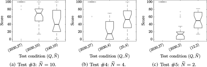
Box plot of scores showing truncation and sparsity conditions at different SH orders, for loudness stability evaluation. Each box represents a different \((Q,\widetilde {N})\) condition. The box bounds the IQR divided by the median, and Tukey-style whiskers extend to a maximum of 1.5 × IQR beyond the box. The notches refer to a 95% confidence interval. a Test #3: \(\widetilde {N} = 10\). b Test #4: \(\widetilde {N} = 4\). c Test #5: \(\widetilde {N} = 2\)

References
H. Møller, Fundamentals of binaural technology. Appl. Acoust.36(3), 171–218 (1992).
M. Kleiner, B. -I. Dalenbäck, P. Svensson, Auralization - an overview. J. Audio Eng. Soc.41(11), 861–875 (1993).
S. M. LaValle, A. Yershova, M. Katsev, M. Antonov, in 2014 IEEE International Conference on Robotics and Automation (ICRA). Head tracking for the oculus rift (IEEEHong Kong, 2014), pp. 187–194.
B. Xie, Head-related transfer function and virtual auditory display (J. Ross Publishing., Plantation, 2013).
J. Blauert, Spatial hearing: the psychophysics of human sound localization (MIT press, Cambridge, 1997).
F. L. Wightman, D. J. Kistler, Headphone simulation of free-field listening. ii: psychophysical validation. J. Acoust. Soc. Am.85(2), 868–878 (1989).
H. Møller, M. F. Sørensen, D. Hammershøi, C. B. Jensen, Head-related transfer functions of human subjects. J. Audio Eng. Soc.43(5), 300–321 (1995).
A. Andreopoulou, D. R. Begault, B. F. Katz, Inter-laboratory round robin HRTF measurement comparison. IEEE J. Sel. Top. Sign. Process.9(5), 895–906 (2015).
E. M. Wenzel, M. Arruda, D. J. Kistler, F. L. Wightman, Localization using nonindividualized head-related transfer functions. J. Acoust. Soc. Am.94(1), 111–123 (1993).
D. R. Begault, E. M. Wenzel, M. R. Anderson, Direct comparison of the impact of head tracking, reverberation, and individualized head-related transfer functions on the spatial perception of a virtual speech source. J. Audio Eng. Soc.49(10), 904–916 (2001).
P. Majdak, P. Balazs, B. Laback, Multiple exponential sweep method for fast measurement of head-related transfer functions. J. Audio Eng. Soc.55(7/8), 623–637 (2007).
A. W. Bronkhorst, Localization of real and virtual sound sources. J. Acoust. Soc. Am.98(5), 2542–2553 (1995).
D. R. Begault, L. J. Trejo, 3-D sound for virtual reality and multimedia (NASA, Ames Research Center, Moffett Field, California, 2000).
M. Noisternig, T. Musil, A. Sontacchi, R. Höldrich, in Proceedings of the 2003 International Conference on Auditory Display. A 3D real time rendering engine for binaural sound reproduction (Georgia Institute of TechnologyBoston, 2003), pp. 107–110.
P. Runkle, M. Blommer, G. Wakefield, in Applications of Signal Processing to Audio and Acoustics, 1995., IEEE ASSP Workshop On. A comparison of head related transfer function interpolation methods (IEEENew Paltz, 1995), pp. 88–91.
K. Hartung, J. Braasch, S. J. Sterbing, in Audio Engineering Society Conference: 16th International Conference: Spatial Sound Reproduction. Comparison of different methods for the interpolation of head-related transfer functions (Audio Engineering Society, 1999), pp. 319–329.
M. J. Evans, J. A. Angus, A. I. Tew, Analyzing head-related transfer function measurements using surface spherical harmonics. J. Acoust. Soc. Am.104(4), 2400–2411 (1998).
G. D. Romigh, D. S. Brungart, R. M. Stern, B. D. Simpson, Efficient real spherical harmonic representation of head-related transfer functions. IEEE J. Sel. Top. Signal Process.9(5), 921–930 (2015).
B. Rafaely, B. Weiss, E. Bachmat, Spatial aliasing in spherical microphone arrays. IEEE Trans. Signal Process.55(3), 1003–1010 (2007).
A. Avni, J. Ahrens, M. Geier, S. Spors, H. Wierstorf, B. Rafaely, Spatial perception of sound fields recorded by spherical microphone arrays with varying spatial resolution. J. Acoust. Soc. Am.133(5), 2711–2721 (2013).
B. Rafaely, Fundamentals of spherical array processing, vol. 8 (Springer, Cham, 2015).
R. Duraiswami, D. N. Zotkin, Z. Li, E. Grassi, N. A. Gumerov, L. S. Davis, in 119th Convention of Audio Engineering Society. High order spatial audio capture and binaural head-tracked playback over headphones with HRTF cues (Audio Engineering Society (AES)New York, 2005).
J. Sheaffer, S. Villeval, B. Rafaely, in Proc. of the EAA Joint Symposium on Auralization and Ambisonics. Rendering binaural room impulse responses from spherical microphone array recordings using timbre correction (Universitätsverlag der TU BerlinBerlin, 2014).
Z. Ben-Hur, F. Brinkmann, J. Sheaffer, S. Weinzierl, B. Rafaely, Spectral equalization in binaural signals represented by order-truncated spherical harmonics. J. Acoust. Soc. Am.141(6), 4087–4096 (2017).
F. Rumsey, Spatial quality evaluation for reproduced sound: terminology, meaning, and a scene-based paradigm. J. Audio Eng. Soc.50(9), 651–666 (2002).
C. Guastavino, B. F. Katz, Perceptual evaluation of multi-dimensional spatial audio reproduction. J. Acoust. Soc. Am.116(2), 1105–1115 (2004).
Z. Ben-Hur, D. L. Alon, B. Rafaely, R. Mehra, Perceived stability and localizability in binaural reproduction with sparse HRTF measurement grids. J. Acoust. Soc. Am.143(3), 1824–1824 (2018).
D. L. Alon, Z. Ben-Hur, B. Rafaely, R. Mehra, in 2018 IEEE International Conference on Acoustics, Speech and Signal Processing (ICASSP). Sparse head-related transfer function representation with spatial aliasing cancellation (IEEECalgary, 2018), pp. 6792–6796.
F. Brinkmann, S. Weinzierl, in Audio Engineering Society Conference: 2018 AES International Conference on Audio for Virtual and Augmented Reality. Comparison of head-related transfer functions pre-processing techniques for spherical harmonics decomposition (Audio Engineering SocietyRedmond, 2018).
D. N. Zotkin, R. Duraiswami, N. A. Gumerov, in 2009 IEEE Workshop on Applications of Signal Processing to Audio and Acoustics. Regularized HRTF fitting using spherical harmonics (IEEENew Paltz, 2009), pp. 257–260.
W. Zhang, T. D. Abhayapala, R. A. Kennedy, R. Duraiswami, Insights into head-related transfer function: spatial dimensionality and continuous representation. J. Acoust. Soc. Am.127(4), 2347–2357 (2010).
M. Aussal, F. Alouges, B. Katz, in Proceedings of Meetings on Acoustics, vol. 19. A study of spherical harmonics interpolation for HRTF exchange (Acoustical Society of AmericaMontreal, 2013), p. 050010.
P. Guillon, R. Nicol, L. Simon, in Audio Engineering Society Convention 125. Head-related transfer functions reconstruction from sparse measurements considering a priori knowledge from database analysis: a pattern recognition approach (Audio Engineering SocietySan Francisco, 2008).
W. Zhang, R. A. Kennedy, T. D. Abhayapala, Efficient continuous HRTF model using data independent basis functions: experimentally guided approach. IEEE Trans. Audio Speech Lang. Process.17(4), 819–829 (2009).
B. Rafaely, A. Avni, Interaural cross correlation in a sound field represented by spherical harmonics. J. Acoust. Soc. Am.127(2), 823–828 (2010).
G. B. Arfken, H. J. Weber, Mathematical methods for physicists (Academic Press, San Diego, 2001).
B. Rafaely, Analysis and design of spherical microphone arrays. Speech Audio Process. IEEE Trans.13(1), 135–143 (2005).
G. F. Kuhn, Model for the interaural time differences in the azimuthal plane. J. Acoust. Soc. Am.62(1), 157–167 (1977).
C. P. Brown, R. O. Duda, A structural model for binaural sound synthesis. IEEE Trans. Speech Audio Process.6(5), 476–488 (1998).
Z. Ben-Hur, J. Sheaffer, B. Rafaely, Joint sampling theory and subjective investigation of plane-wave and spherical harmonics formulations for binaural reproduction. Appl. Acoust.134(1), 138–144 (2018).
M. Burkhard, R. Sachs, Anthropometric manikin for acoustic research. J. Acoust. Soc. Am.58(1), 214–222 (1975).
B. Bernschütz, in Proceedings of the 40th Italian (AIA) Annual Conference on Acoustics and the 39th German Annual Conference on Acoustics (DAGA) Conference on Acoustics. A spherical far field HRIR/HRTF compilation of the Neumann KU 100 (AIA/DAGAMerano, 2013), p. 29.
F. Brinkmann, A. Lindau, S. Weinzierl, S. van de Par, M. Müller-Trapet, R. Opdam, M. Vorländer, A High Resolution and Full- Spherical Head-Related Transfer Function Database for Different Head-Above- Torso Orientations. J. Audio Eng. Soc. 65(10), 841–848 (2017).
T. Huttunen, A. Vanne, in Audio Engineering Society Convention 142. End-To-End process for HRTF personalization, (2017).
V. Lebedev, D. Laikov, in Doklady. Mathematics, vol. 59. A quadrature formula for the sphere of the 131st algebraic order of accuracy (MAIK Nauka/Interperiodica, 1999), pp. 477–481.
R. H. Hardin, N. J. Sloane, Mclarens improved snub cube and other new spherical designs in three dimensions. Discret. Comput. Geom.15(4), 429–441 (1996).
I. H. Sloan, R. S. Womersley, Extremal systems of points and numerical integration on the sphere. Adv. Comput. Math.21(1-2), 107–125 (2004).
M. Slaney, Auditory toolbox version 2. Interval research corporation. Indiana Purdue Univ.2010:, 1998–010 (1998).
J. P. Boyd, Chebyshev and Fourier Spectral Methods (Courier Corporation, Mineola, 2001).
R. O. Duda, W. L. Martens, Range dependence of the response of a spherical head model. J. Acoust. Soc. Am.104(5), 3048–3058 (1998).
ITU-R-BS.1770-4, Algorithms to measure audio programme loudness and true-peak audio level (Electronic Publication, Geneva, 2015).
B. Rafaely, M. Kleider, Spherical microphone array beam steering using Wigner-D weighting. Signal Process. Lett. IEEE.15:, 417–420 (2008).
H. Møller, D. Hammershøi, C. B. Jensen, M. F. Sørensen, Transfer characteristics of headphones measured on human ears. J. Audio Eng. Soc.43(4), 203–217 (1995).
D. Pralong, S. Carlile, The role of individualized headphone calibration for the generation of high fidelity virtual auditory space. J. Acoust. Soc. Am.100(6), 3785–3793 (1996).
J. Ahrens, M. Geier, S. Spors, in Audio Engineering Society Convention 124. The soundscape renderer: a unified spatial audio reproduction framework for arbitrary rendering methods (Audio Engineering SocietyAmsterdam, 2008).
S. Yairi, Y. Iwaya, Y. Suzuki, Influence of large system latency of virtual auditory display on behavior of head movement in sound localization task. Acta Acustica United Acustica.94(6), 1016–1023 (2008).
N. Sankaran, J. Hillis, M. Zannoli, R. Mehra, Perceptual thresholds of spatial audio update latency in virtual auditory and audiovisual environments. J. Acoust. Soc. Am.140(4), 3008–3008 (2016).
Z. Schärer, A. Lindau, in Audio Engineering Society Convention 126. Evaluation of equalization methods for binaural signals (Audio Engineering SocietyMunich, 2009).
ITU-R-BS, 1534-1: Method for the subjective assessment of intermediate quality level of coding systems (Electronic Publication, Geneva, 2003).
ITU-R-BS, 1534-3: Method for the subjective assessment of intermediate quality level of audio systems (Electronic Publication, Geneva, 2015).
J. Breebaart, Evaluation of statistical inference tests applied to subjective audio quality data with small sample size. IEEE/ACM Trans. Audio Speech Lang. Process. (TASLP).23(5), 887–897 (2015).
B. Bernschütz, A. V. Giner, C. Pörschmann, J. Arend, Binaural reproduction of plane waves with reduced modal order. Acta Acustica United Acustica.100(5), 972–983 (2014).
J. W. Tukey, Exploratory data analysis, vol. 2 (Addison-Wesley, Reading, Massachusetts, 1977).
Acknowledgements
Not applicable.
Funding
This research was supported in part by Facebook Reality Labs and Ben-Gurion University of the Negev.
Availability of data and materials
The datasets used and analyzed during the current study are available from the corresponding author on reasonable request.
Author information
Authors and Affiliations
Contributions
ZB performed the entire research and its writing. DA supported the experimental part, and BR and RM supervised the research. All authors read and approved the final manuscript.
Corresponding author
Ethics declarations
Competing interests
The authors declare that they have no competing interests.
Publisher’s Note
Springer Nature remains neutral with regard to jurisdictional claims in published maps and institutional affiliations.
Rights and permissions
Open Access This article is distributed under the terms of the Creative Commons Attribution 4.0 International License (http://creativecommons.org/licenses/by/4.0/), which permits unrestricted use, distribution, and reproduction in any medium, provided you give appropriate credit to the original author(s) and the source, provide a link to the Creative Commons license, and indicate if changes were made.
About this article

Cite this article
Ben-Hur, Z., Alon, D., Rafaely, B. et al. Loudness stability of binaural sound with spherical harmonic representation of sparse head-related transfer functions. J AUDIO SPEECH MUSIC PROC. 2019, 5 (2019). https://doi.org/10.1186/s13636-019-0148-x
Received:
Accepted:
Published:
DOI: https://doi.org/10.1186/s13636-019-0148-x