A simulation study on optimal scores for speaker recognition

Abstract

In this article, we conduct a comprehensive simulation study for the optimal scores of speaker recognition systems that are based on speaker embedding. For that purpose, we first revisit the optimal scores for the speaker identification (SI) task and the speaker verification (SV) task in the sense of minimum Bayes risk (MBR) and show that the optimal scores for the two tasks can be formulated as a single form of normalized likelihood (NL). We show that when the underlying model is linear Gaussian, the NL score is mathematically equivalent to the PLDA likelihood ratio (LR), and the empirical scores based on cosine distance and Euclidean distance can be seen as approximations of this linear Gaussian NL score under some conditions.Based on the unified NL score, we conducted a comprehensive simulation study to investigate the behavior of the scoring component on both the SI task and SV task, in the case where the distribution of the speaker vectors perfectly matches the assumption of the NL model, as well as the case where some mismatch is involved. Importantly, our simulation is based on the statistics of speaker vectors derived from a practical speaker recognition system, hence reflecting the behavior of the NL scoring in real-life scenarios that are full of imperfection, including non-Gaussianality, non-homogeneity, and domain/condition mismatch.

1 Introduction

With decades of investigation, speaker recognition has achieved significant performance and has been deployed in a wide range of practical applications [1–3]. Speaker recognition research concerns two tasks: speaker identification (SI) that identify the true speaker from a set of candidates, and speaker verification (SV) that tests if an alleged speaker is the true speaker. The performance of SI systems is evaluated by identification rate (IDR), the percentage of the trials whose speakers are correctly identified. SV systems require a threshold to decide whether accepting the speaker or not and the performance is evaluated by equal error rate (EER), to represent the trade-off between fail to accept and fail to reject.

Modern speaker recognition methods are based on the concept of speaker embedding, i.e., representing speakers by fixed-length continuous speaker vectors. This embedding is traditionally based on statistical models, in particular the i-vector model [4]. Recently, deep learning methods gained much attention and embedding based on deep neural nets (DNN) becomes popular [5, 6]. With the efforts from multiple research groups, deep speaker embedding models have been significantly improved by comprehensive architectures [7, 8], smart pooling approaches [9–12], task-oriented objectives [13–18], and carefully designed training schemes [19–21]. As a result, the deep embedding approach has achieved state-of-the-art performance [22]. Among various deep embedding architectures, the x-vector model is the most popular [23].

A key component of the speaker embedding approach is how to score a trial. Numerous empirical evidence has shown that the likelihood ratio (LR) derived by probabilistic linear discriminant analysis (PLDA) [24, 25] works well in most situations, and when the computational resource is limited, the cosine distance is a reasonable substitution. In some circumstances in particular on SI tasks, the Euclidean distance can be used. In this article, we revisit the scoring methods for speaker recognition from the perspective of minimum Bayes risk (MBR). The analysis shows that for both the SI and SV tasks, the MBR optimal score can be formulated as a single form $\frac {p_{k}(\boldsymbol {x})}{p(\boldsymbol {x})}$, which we call a normalized likelihood (NL) score. In the NL score, p_k(x) is the likelihood term that represents the probability that the test utterance x belongs to the target class k, and p(x) is a normalization term that represents the probability that x belongs to all possible classes. We will show that the NL score is equivalent to PLDA LR, in the case where the speaker vectors are modeled by a linear Gaussian and the target class is represented by finite enrollment utterances. We will also show that under some conditions, the empirical scores based on cosine distance and Euclidean distance can be derived from the linear Gaussian NL score.

Based on the unified formulation of the NL score, we conducted a comprehensive simulation study on the performance bound of a speaker recognition system, on both the SI and SV tasks. In particular, by imitating the statistical properties of speaker vectors derived from a real recognition system, our simulation gained deep understanding of a modern speaker recognition system, for instance the upper bound of its performance, and its behavior with real-life imperfection, including non-Gaussianality, non-homogeneity, training-deployment domain mismatch, and enrollment-test condition mismatch. To the best knowledge of the author, this is the first comprehensive simulation study on the scoring component of modern speaker recognition systems. Note that the NL formulation is a prerequisite for the simulation study: it not only allows using the same score to investigate the behavior of both the SI and SV systems, but also offers the possibility to decompose the scoring model into separate components (by using different statistical models), which is important when we analyze the domain and condition mismatch.

It should be noted that the NL formulation is not new and may trace back to the LR scoring method with the Gaussian mixture model-universal background model (GMM-UBM) framework [26]. Within the speaker embedding framework, the NL form was derived by McCree et. al. [27, 28] from the hypothesis test view (the one used for PLDA inference). Our derivation is based on the MBR decision theory, which directly affirms the optimum of the NL score.

The rest of the paper is organized as follows: Section 2 will revisit the MBR optimal scoring theory and propose the NL score. Section 3 presents the simulation results. Some discussions are presented in Section 4, and the entire paper is concluded in Section 5.

2 Theory and methods

2.1 MBR optimal decision and normalized likelihood

It is well known that an optimal decision for a classification task should minimize the Bayes risk (MBR):

$$ k^{*} = \arg\min_{k} \sum_{j} \ell_{{jk}} p(j|\boldsymbol{x}) $$

(1)

where x is the observation, ℓ_jk is the risk taken when classifying an observation from class j to class k. In the case where ℓ_jk is 0 for j=k and a constant c for any j≠k, the MBR decision is equal to selecting the class with the largest posterior probability:

$$ k^{*} = \arg\max_{k} p(k|\boldsymbol{x}). $$

(2)

We call this result the MAP principle. We will employ this principle to derive the optimal score for the SI and SV tasks in speaker recognition.

2.1.1 MBR optimal score for SI

In the SI task, our goal is to test K outcomes {H_k: x belongs to class k} and make the decision which outcome is the most probable. Following the MAP principle, the MBR optimal decision is to choose the kth outcome that obtains the maximum posterior:

$$ k^{*} = \arg\max_{k} p(H_{k}|\boldsymbol{x}) = \arg\max_{k} p_{k}(\boldsymbol{x}) p(k), $$

(3)

where k indexes the classes, and p_k(x) represents the likelihood of x in class k. In most cases, there is no preference for any particular class and so the prior p(k) for each class k shall be equal. We therefore have:

$$ k^{*} = \arg\max_{k} p_{k}(\boldsymbol{x}). $$

(4)

It indicates that MBR optimal decisions can be conducted based on the likelihood p_k(x). In other words, the likelihood is MBR optimal for the SI task.

2.1.2 MBR optimal score for SV

For the SV task, our goal is to test two outcomes and check which one is more probable: {H₀:x belongs to class k;H₁:xbelongs to any class other thank}. Following the MAP principle, the MBR optimal decision should be based on the posterior p(H_b|x):b={0,1}, if the risk for H₀ and H₁ is symmetric. If the priors p(H₀) and p(H₁) are equal, we have:

$$ p(H_{b}|\boldsymbol{x}) = \frac{p(\boldsymbol{x}|H_{b})}{p(\boldsymbol{x}|H_{0}) + p(\boldsymbol{x}|H_{1})}. $$

(5)

Since p(H₀|x)+p(H₁|x)=1, the decision can be simply made according to p(H₀|x):

$$ b^{*} = \left\{\begin{array}{ll} 0 & if \ p(H_{0}|\boldsymbol{x}) \ge 0.5\\ 1 & if \ p(H_{0}|\boldsymbol{x}) < 0.5. \end{array}\right. $$

(6)

In practice, by setting an appropriate threshold on p(H₀|x), one can deal with different priors and risk on H₀ and H₁. We highlight that for any class k, this threshold is only related to the prior and risk. This is important as it means that based on p(H₀|x), MBR optimal decisions can be made simultaneously for all the classes by setting a global threshold. A simple case is to set the threshold to 0.5 when the risk is symmetric and the priors are equal. In summary, p(H₀|x) is MBR optimal for the SV task.

Note that when computing the posterior p(H₀|x),p(x|H₀) is exactly the likelihood p_k(x), and p(x|H₁) summarizes the likelihood of all possible classes except the class k. In most cases, an SV system is required to deal with any unknown class, and so the class space is usually assumed to be continuous. To simplify the presentation, we will assume each class being uniquely represented by the mean vector μ and p(μ) is continuous. In this case, the contribution of each class is infinitely small and so p(x|H₁) is exactly the marginal distribution (or evidence) $p(\boldsymbol {x})=\int p(\boldsymbol {x}|\boldsymbol {\mu }) p(\boldsymbol {\mu })\mathrm {d} \boldsymbol {\mu }$¹. We therefore obtain the MBR optimal score for SV:

$$ p(H_{0}|\boldsymbol{x}) = \frac{p_{k}(\boldsymbol{x})}{p_{k}(\boldsymbol{x}) + p(\boldsymbol{x})}. $$

(7)

2.1.3 Normalized likelihood

Note that for the SV task, according to Eq.(5), the posterior p(H₀|x) is determined by the ratio p(x|H₀)/p(x|H₁), which is essentially the class-dependent likelihood p_k(x) normalized by the class-independent likelihood p(x). We therefore define the normalized likelihood (NL) as:

$$ NL (\boldsymbol{x}|k)= \frac{p(\boldsymbol{x}|H_{0})}{p(\boldsymbol{x}|H_{1})} = \frac{p_{k}(\boldsymbol{x})}{p(\boldsymbol{x})}. $$

(8)

Note that the NL is linked to the posterior p(H₀|x) by a monotone function:

$$ NL (\boldsymbol{x} |k) = \frac{p(H_{0}|\boldsymbol{x})}{1 - p(H_{0}|\boldsymbol{x})}. $$

(9)

Since the posterior p(H₀|x) is MBR optimal for the SV task, the NL is also MBR optimal as a threshold on p(H₀|x) that leads to (global) MBR decisions can be simply transformed to a threshold on the NL, by which the same MBR decisions can be achieved. For example, the MBR decision is obtained when p(H₀|x)=0.5 if the risk on H₀ and H₁ is equal, which is equal to say NL(x|k)=1.0, according to Eq.(9).

Interestingly, the NL score is also MBR optimal for the SI task. This is because the normalization term p(x) is the same for all classes in the SI task, so the decisions made based on the NL score is equal to those based on the likelihood p_k(x). Since the likelihood is MBR optimal for the SI task, the NL score is MBR optimal for the SI task as well. We therefore conclude that the NL score is MBR optimal for both the SI and the SV tasks, under some appropriate assumptions. It should be noted that the NL form Eq. (8) is a high-level definition and it can be implemented in a flexible way. In particular, p_k(x) and p(x) can be any models that produce the class-dependent and class-independent likelihoods respectively.

Finally, NL is not new for speaker recognition. It is essentially the likelihood ratio (LR) that has been employed for many years since the GMM-UBM regime, where the score is computed by $\frac {p_{{GMM}}(\boldsymbol {x})}{p_{{UBM}}(\boldsymbol {x})}$. We use the term NL instead of LR in this paper in order to (1) highlight the different roles of the numerator p_k(x) and the denominator p(x) in the ratio and (2) discriminate the normalization-style LR (used by NL) and the comparison-style LR, e.g., the one used by PLDA inference that compares the likelihoods that a group of samples are generated from the same and different classes.

2.2 NL score with linear Gaussian model

Although the NL framework allows flexible models for the class-dependent and class-independent likelihoods, linear Gaussian model is the most attractive due to its simplicity. We derive the NL score with this model; for case (1), the class means have been known and (2) the class means are unknown and have to be estimated from enrollment data.

2.2.1 Linear Gaussian model

We shall assume a simple linear Gaussian model for the speaker vectors that we will score:

$$ p(\boldsymbol{\mu}) = N\left(\boldsymbol{\mu}; \boldsymbol{0}, \mathbf{I} \boldsymbol{\epsilon}^{2} \right) $$

(10)

$$ p(\boldsymbol{x}|\boldsymbol{\mu}) = N\left(\boldsymbol{x}; \boldsymbol{\mu}, \sigma^{2} \mathbf{I}\right), $$

(11)

where μ∈R^D represents the means of classes and x∈R^D represents observations, and ε²∈(R⁺)^D and σ²∈R⁺ represent the between-class and within-class variances respectively. Applied to speaker recognition, ε and σ represent the between-speaker and within-speaker variances respectively. We highlight that any linear Gaussian model can be transformed into this simple form (i.e., isotropic within-class covariance and diagonal between-class covariance) by a linear transform such as full-dimensional linear discriminant analysis (LDA), and this linear transform will not change the identification and verification results as we will show in Section 2.3. Therefore, study with the simple form Eqs. (10) and (11) is sufficient for us to understand the behavior of a general linear Gaussian model with complex covariance matrices.

With this model, it is easy to derive the marginal probability p(x) and the posterior probability p(μ|x) as follows [29]:

$$ p(\boldsymbol{x}) = N\left(\boldsymbol{x}; \boldsymbol{0}, \mathbf{I} \left(\boldsymbol{\epsilon}^{2} + \sigma^{2}\right) \right) $$

(12)

$$ p(\boldsymbol{\mu}|\boldsymbol{x}) = N\left(\boldsymbol{\mu}; \frac{\boldsymbol{\epsilon}^{2}}{\boldsymbol{\epsilon}^{2} + \sigma^{2}} \boldsymbol{x}, \mathbf{I} \frac{\sigma^{2} \boldsymbol{\epsilon}^{2}}{\boldsymbol{\epsilon}^{2} + \sigma^{2}} \right), $$

(13)

where all the operations between vectors are element-wised and appropriate dimension expansion has been assumed, e.g., ε²+σ²=ε²+[σ²,...,σ²]^T.

If the observations are more than one, the posterior probability has the form:

$$ p\left(\boldsymbol{\mu}|\boldsymbol{x}_{1},...,\boldsymbol{x}_{n}\right) = N\left(\boldsymbol{\mu}; \frac{n \boldsymbol{\epsilon}^{2}}{n\boldsymbol{\epsilon}^{2} + \sigma^{2}} \bar{\boldsymbol{x}}, \mathbf{I} \frac{ \sigma^{2} \boldsymbol{\epsilon}^{2}}{n\boldsymbol{\epsilon}^{2} + \sigma^{2}} \right), $$

(14)

where $\bar {\boldsymbol {x}}$ is the average of the observations. These equations will be extensively used in the following sections.

2.2.2 Case 1: class means are known

In this case, we assume that the class means are known. This is equivalent to say that each class is represented by infinite enrollment data.

NL/Euclidean/Cosine scores for SI

For the SI tasks, decisions based on the NL score and the likelihood p_k(x) are the same and both are MBR optimal. With the linear Gaussian model, the likelihood is:

$$ p_{k}(\boldsymbol{x}) = N\left(\boldsymbol{x}; \boldsymbol{\mu}_{k}, \sigma^{2} \mathbf{I}\right). $$

(15)

A simple rearrangement shows that:

$$ \log p_{k}(\boldsymbol{x}) = -\frac{1}{2 \sigma^{2}} \left\|\boldsymbol{x} - \boldsymbol{\mu}_{k}\right\|^{2} + const $$

(16)

Since the variance σ is the same for all classes, the MBR decision can be equally based on the Euclidean distance, e.g.,

$$ s_{e} = \left\|\boldsymbol{x} - \boldsymbol{\mu}_{k}\right\|^{2}, $$

(17)

where we use s_e to denote the score based on the Euclidean distance. In short, the Euclidean score is MBR optimal for the SI task when the class means are known.

Next, we will show that in a high-dimensional space, the Euclidean distance is well approximated by the cosine distance, under the linear Gaussian assumption.

First notice that the Gaussian annulus theorem [30] states that for a d-dimensional Gaussian distribution with the same variance ε in each direction, nearly all the probability mass is concentrated in a thin annulus of width O(1) at radius $\sqrt {d}\epsilon$, as shown in Fig. 1. This slightly anti-intuitive result indicates that in a high-dimensional space, most of the samples from a Gaussian tend to be in the same length. Rigid proof for this theorem can be found in [30]. Note that the distribution of real speaker vectors is not necessarily a perfect Gaussian; however, in most cases, it can be well approximated by a Gaussian, especially when some normalization techniques are employed [31]. Therefore, the Gaussian annulus theorem can be readily used for speaker vectors.

Fig. 1

Left: Gaussian annulus theorem [30]: for a d-dimensional multi-variant Gaussian with unit variance in all directions, for any $\beta \le \sqrt {d}$, all but at most $3e^{-c\beta ^{2}}$ of the probability mass lies within the annulus $\sqrt {d}-\beta \le \|{x}\| \le \sqrt {d} + \beta$, where c is a fixed positive constant. The color region shown in the figure represents the annulus. Rigid proof can be found in [30]. Right: The length distribution of samples from a 512-dimensional Gaussian distribution N(0,I)

Now we rewrite the Euclidean score as follows:

$$ s_{e} = \|\boldsymbol{x}\|^{2} + \|\boldsymbol{\mu}_{k}\|^{2} - 2 \cos \left(\boldsymbol{x}, \boldsymbol{\mu}_{k}\right) \|\boldsymbol{x}\| \ \|\boldsymbol{\mu}_{k}\|, $$

(18)

since $\|\boldsymbol {\mu }_{k}\| \approx \sqrt {d}\epsilon, \cos \left (\boldsymbol {x}, \boldsymbol {\mu }_{k}\right)$ will be the only term that discriminates the probability that x belongs to different class k. This leads to the cosine score:

$$ s_{c} = \cos (\boldsymbol{x}, \boldsymbol{\mu}_{k}). $$

(19)

This result provides the theoretical support for the cosine score. It should be noted that this approximation is only valid for high-dimensional data, and the class means must be from a Gaussian with a zero mean. Therefore, data centralization is important for cosine scoring.

NL/Euclidean/Cosine scores for SV

For the SV task, the MBR optimal decision should be based on the NL score. With the linear Gaussian model, one can easily show that:

$$ {}\log NL (\boldsymbol{x}|k) = -\frac{1}{2 \sigma^{2}} \|\boldsymbol{x} - \boldsymbol{\mu}_{k}\|^{2} + \frac{1}{2}\left\|\frac{\boldsymbol{x}}{\sqrt{\boldsymbol{\epsilon}^{2} + \sigma^{2}}} \right\|^{2} + \ const. $$

(20)

A simple rearrangement shows that:

$$ \begin{aligned} \log NL (\boldsymbol{x} |k) &= -\frac{1}{2\sigma^{2}} \left(\left\|\boldsymbol{x}\right\|^{2} + \left\|\boldsymbol{\mu}_{k}\right\|^{2} - 2 \cos \left(\boldsymbol{x}, \boldsymbol{\mu}_{k}\right) \left\|\boldsymbol{x}\right\| \ \left\|\boldsymbol{\mu}_{k}\right\|\right) \\&\quad+ \frac{1}{2}\left\|\frac{\boldsymbol{x}}{\sqrt{\boldsymbol{\epsilon}^{2} + \sigma^{2}}} \right\|^{2} + \ const \\ &\propto - \left\{ \left\|\frac{\boldsymbol{\epsilon}}{\sqrt{\sigma^{2}+\boldsymbol{\epsilon}^{2}}} \boldsymbol{x}\right\|^{2} \,+\, \left\|\boldsymbol{\mu}_{k}\right\|^{2} - 2 \cos (\boldsymbol{x}, \boldsymbol{\mu}_{k}) \left\|\boldsymbol{x}\right\| \ \left\|\boldsymbol{\mu}_{k}\right\| \right\}. \end{aligned} $$

(21)

It can be seen that if the within-class variance σ² is significantly larger than the between-class variance ε² (we refer to element-based comparison here and after), the logNL will significantly depart from the Euclidean distance, but more closely related to the cosine distance. Essentially, if we admit that both ∥x∥² and ∥μ_k∥² tend to be constant due to the Gaussian annulus theorem, the cosine score will be a good approximation for the optimal logNL. Conversely, if the between-class variance ε² is sufficient larger than the within-class variance σ², it can be well approximated by the Euclidean score.

2.2.3 Case 2: class means are unknown

In the pervious section, we have supposed that the class means are known precisely. In real scenarios, however, this is not possible. We usually have only a few enrollment samples (e.g., less than 3) to represent the class, and the SI or SV evaluation should be based on these representative samples. In this case, the class means are unknown and have to be estimated from the enrollment data, leading to uncertainty that must be taken into account during scoring.

NL/Euclidean/Cosine scores for SI

Firstly consider the MBR optimal decision for SI. As in the known-mean scenario, we compute the likelihood for the kth class:

$$ p_{k}(\boldsymbol{x}) = N\left(\boldsymbol{x}; \boldsymbol{\mu}_{k}, \sigma^{2} \mathbf{I}\right). $$

(22)

An important difference here is that μ_k is unknown and so has to be estimated from the enrollment samples belonging to the same class. Denoting these samples by $\boldsymbol {x}^{k}_{1},...\boldsymbol {x}^{k}_{n_{k}}$ and their average by $\bar {\boldsymbol {x}}_{k}$, we have the posterior probability for the class mean μ_k, according to Eq. (14):

$$ {}p\left(\boldsymbol{\mu}_{k} |\boldsymbol{x}^{k}_{1},...\boldsymbol{x}^{k}_{n_{k}} \right) = N\left(\boldsymbol{\mu}_{k} ; \frac{n_{k}\boldsymbol{\epsilon}^{2}}{n_{k}\boldsymbol{\epsilon}^{2} + \sigma^{2}} \bar{\boldsymbol{x}}_{k}, \mathbf{I} \frac{\sigma\boldsymbol{\epsilon}^{2}}{n_{k}\boldsymbol{\epsilon}^{2} + \sigma^{2}} \right). $$

(23)

The likelihood p_k(x) can therefore be computed by marginalizing over μ_k, according to this posterior. Following Eq.(12), we have:

$$\begin{array}{@{}rcl@{}} {}p_{k}(\boldsymbol{x}) &=&p\left(\boldsymbol{x}|\boldsymbol{x}^{k}_{1},..., \boldsymbol{x}^{k}_{n_{k}}\right) \\ &=& \int p(\boldsymbol{x}| \boldsymbol{\mu}_{k}) p\left(\boldsymbol{\mu}_{k}|\boldsymbol{x}^{k}_{1},...\boldsymbol{x}^{k}_{n_{k}}\right) \mathrm{d} \boldsymbol{\mu}_{k} \\ &=& N\left(\boldsymbol{x}; \frac{n_{k}\boldsymbol{\epsilon}^{2}}{n_{k}\boldsymbol{\epsilon}^{2} + \sigma^{2}} \bar{\boldsymbol{x}}_{k}, \left(\sigma^{2} + \mathbf{I} \frac{\sigma\boldsymbol{\epsilon}^{2}}{n_{k}\boldsymbol{\epsilon}^{2} + \sigma^{2}}\right) \right). \end{array} $$

(24)

Note that with the class mean uncertainty, the Euclidean score is not MBR optimal anymore. If the number of enrollment observations are the same for all classes, the likelihood is exclusively determined by the class mean μ_k. In this case, an amended version of the Euclidean score is optimal, where the class mean is computed by $\frac {n_{k}\boldsymbol {\epsilon }^{2}}{n_{k}\boldsymbol {\epsilon }^{2} + \sigma ^{2}}\boldsymbol {\mu }_{k}$. Note that the scale $\frac {n_{k}\boldsymbol {\epsilon }^{2}}{n_{k}\boldsymbol {\epsilon }^{2} + \sigma ^{2}}$ has been applied to compensate for the uncertainty of the maximum-likelihood mean estimation μ_k. Intuitively, a smaller n or a larger σ²/ε² lead to more uncertainty, so the compensation term will be more significant. With more enrollment samples, the compensation term will converge to one, and the standard Euclidean score is recovered.

Another observation is that the scale compensation on μ_k does not change its direction. This implies that the cosine score does not need any amendment to account for the uncertainty. However, it does not mean that the cosine score is not impacted by the class mean uncertainty; it just means that the cosine score is not impacted as much as the Euclidean score.

NL/Euclidean/Cosine scores for SV

Now, we normalize the score p_k(x) to make it suitable for SV, by introducing a normalization term p(x):

$$\begin{array}{@{}rcl@{}} NL (\boldsymbol{x} |k)= \frac{p\left(\boldsymbol{x}|\boldsymbol{x}_{1},..., \boldsymbol{x}_{n_{k}}\right)} {p(\boldsymbol{x})}. \end{array} $$

(25)

Note that the normalization term p(x) is not impacted by the mean uncertainty and therefore remains the same value as in the known-mean scenario. A simple computation shows that:

$$ \log NL (\boldsymbol{x} |k) \propto -\left\|\frac{\boldsymbol{x} - \tilde{\boldsymbol{\mu}}_{k}}{\sqrt{\sigma^{2} + \frac{\boldsymbol{\epsilon}^{2} \sigma^{2}}{n_{k} \boldsymbol{\epsilon}^{2} + \sigma^{2}}}} \right\|^{2} + \left\|\frac{\boldsymbol{x}}{\sqrt{\boldsymbol{\epsilon}^{2} + \sigma^{2}}} \right\|^{2}, $$

(26)

where we have defined:

$$ \tilde{\boldsymbol{\mu}}_{k} = \frac{n_{k}\boldsymbol{\epsilon}^{2}}{n_{k}\boldsymbol{\epsilon}^{2} + \sigma^{2}} \bar{\boldsymbol{x}}_{k}. $$

(27)

To compare with the Euclidean score and the cosine score, Eq. (25) can be reformulated to:

$$ {}\begin{aligned} \log NL (\boldsymbol{x} |k) &\propto - \left\{\frac{n_{k} \boldsymbol{\epsilon}^{4}}{\left(\sigma^{2} +\boldsymbol{\epsilon}^{2}\right)\left(n_{k} \boldsymbol{\epsilon}^{2} + \sigma^{2}\right)}\|\boldsymbol{x}\|^{2} + \|\tilde{\boldsymbol{\mu}}_{k}\|^{2}\right.\\ &\quad-\left.{\vphantom{\frac{n_{k} \boldsymbol{\epsilon}^{4}}{\left(\sigma^{2} +\boldsymbol{\epsilon}^{2}\right)\left(n_{k} \boldsymbol{\epsilon}^{2} + \sigma^{2}\right)}}} 2 \cos \left(\boldsymbol{x}, \tilde{\boldsymbol{\mu}}_{k}\right) \|\boldsymbol{x}\| \ \|\boldsymbol{\mu}_{k}\| \right\}. \end{aligned} $$

(28)

It can be seen that if the between-class variance ε is significantly smaller than the within-class variance σ, the first two terms on the right hand side of Eq. (28) tend to be small and logNL can be approximated by the cosine score. On the opposite, if the between-class variance ε is significantly larger than the within-class variance σ, the amended Euclidean score will be a good approximation. Finally, if n_k is sufficiently large, Eq. (28) will fall back to Eq. (21) of the know-mean case.

2.3 Remarks on properties of NL score

Remark 1: Equivalent to PLDA LR

The NL score based on the linear Gaussian model and unknown class means is equivalent to the PLDA LR [24, 25]. PLDA assumes the same linear Gaussian model, but uses the following likelihood ratio as the score:

$$\begin{aligned} {LR}_{{PLDA}} (\boldsymbol{x}) \,=\, \frac{p\left(\boldsymbol{x},\boldsymbol{x}_{1},...,\boldsymbol{x}_{n} \ from \ the \ same \ class \right) }{p (\boldsymbol{x} \ from \ a \ unique \ class) p (\boldsymbol{x_{1},..., x_{n}} \ from \ a \ unique \ class)} \end{aligned} $$

Note that this likelihood ratio is different from the likelihood ratio of the NL score in Eq. (8). The PLDA LR can be formally represented by:

$$ {LR}_{{PLDA}} (\boldsymbol{x}) = \frac{p\left(\boldsymbol{x},\boldsymbol{x}_{1},...,\boldsymbol{x}_{n}\right)}{p (\boldsymbol{x}) p \left(\boldsymbol{x}_{1},..., \boldsymbol{x}_{n}\right)} $$

(29)

where p(x₁,...,x_n) denotes the probability that x₁,...,x_n belong to the same but an unknown class. In principle, this quantity can be computed by marginalizing over the class mean:

$$ p\left(\boldsymbol{x}_{1},..., \boldsymbol{x}_{n}\right) = \int p\left(\boldsymbol{x}_{1},.., \boldsymbol{x}_{n} | \boldsymbol{\mu}\right) p(\boldsymbol{\mu}) \mathrm{d} \boldsymbol{\mu}. $$

(30)

A simple re-arrangement shows that:

$$ {LR}_{{PLDA}} (\boldsymbol{x}) = \frac{p\left(\boldsymbol{x}| \boldsymbol{x}_{1},..., \boldsymbol{x}_{n}\right)}{p(\boldsymbol{x})} \,=\, \frac{\int p(\boldsymbol{x}|\boldsymbol{\mu}) p\left(\boldsymbol{\mu}| \boldsymbol{x}_{1},..., \boldsymbol{x}_{n}\right) \mathrm{d} \boldsymbol{\mu}}{p(\boldsymbol{x})}, $$

(31)

where we have divided the numerator p(x,x₁,...,x_n) by p(x₁,...,x_n), which converts the marginal distribution p(x,x₁,...,x_n) to the conditional distribution p(x|x₁,...,x_n). By this change, the numerator is the likelihood of x belonging to the class represented by x₁,...,x_n, and the denominator is the likelihood x belonging to any class. This is exactly the normalized likelihood in Eq. (25). We therefore conclude that the PLDA LR is an NL where the underlying probabilistic model is linear Gaussian and the class means are estimated from finite enrollment data. Since the NL score is MBR optimal for both SI and SV tasks, an immediate conclusion is that the PLDA LR is also MBR optimal for the two tasks. Note that the NL form of the PLDA LR was discussed by McCree et. al. [27, 28].

Compared to PLDA LR, NL possesses some attractive properties and brings some interesting merits. A particular merit is that NL decouples the score computation into three steps: posterior computation based on enrollment data, likelihood computation for the test data based on the posterior, and normalization based on a global model. This offers an interesting correspondence between the scoring model and the scoring process. We therefore can investigate the behavior of each component and design fine-grained treatment for real-life imperfection, e.g., the enrollment-test mismatch that will be presented in Section 3.7.

Remark 2: Invariance with invertible transform

Suppose an invertible transform g on x, and the probabilities on x and g(x) are p and p^′ respectively. According to the principle of distribution transformation for continuous variables [32], p and p^′ has the following relation:

$$ p'(g(\boldsymbol{x})) = p(\boldsymbol{x}) \left|\det \frac{\partial{g}^{-1}(\boldsymbol{x})}{\partial{\boldsymbol{x}}}\right|, $$

(32)

where the second term is the absolute value of the determinant of the Jacobian matrix of g⁻¹, the inverse transform of g. This term reflects the change of the volume with the transform, and is often called the entropy term and denoted by J(x).

For the marginal distribution p(x₁,...,x_n) where x₁,...,x_n are drawn from the same but an unknown class, one can compute the distribution by:

$$\begin{array}{@{}rcl@{}} p\left(\boldsymbol{x}_{1},..., \boldsymbol{x}_{n}\right) &=& \int \prod_{i=1}^{n} p\left(\boldsymbol{x}_{i} | \boldsymbol{\mu}\right) p(\boldsymbol{\mu}) \mathrm{d} \boldsymbol{\mu} \\ &\approx& \sum_{j} \prod_{i=1}^{n} p(\boldsymbol{x}_{i} | \boldsymbol{\mu}_{j}) p(\boldsymbol{\mu}_{j}) \Delta(\boldsymbol{\mu}_{j}) \end{array} $$

(33)

where we have divide the μ space into a large amount of small areas {Δ(μ_j)} with centers {μ_j}. The approximation will approach to be accurate when the number of small areas is infinite. With the transform g, we have:

$$ \begin{aligned} p'\left(g\left(\boldsymbol{x}_{1}\right),..., g(\boldsymbol{x}_{n})\right) \approx \sum_{j} \prod_{i=1}^{n} p'\left(g\left(\boldsymbol{x}_{i}\right) | \boldsymbol{\mu}^{g}_{j}\right) p'\left(g\left(\boldsymbol{\mu}_{j}\right)\right) \Delta\left(g\left(\boldsymbol{\mu}_{j}\right)\right) \end{aligned} $$

(34)

where $\boldsymbol {\mu }^{g}_{j}$ represents the mean of the class centered at μ_j after the transform. Moreover, the transform g does not change the probability within Δ(μ_j), which means:

$$ p\left(\boldsymbol{\mu}_{j}\right) \Delta\left(\boldsymbol{\mu}_{j}\right) = p'\left(g\left(\boldsymbol{\mu}_{j}\right)\right) \Delta\left(g\left(\boldsymbol{\mu}_{j}\right)\right). $$

(35)

Putting all the pieces together, we have:

$$ \begin{aligned} p'\left(g(\boldsymbol{x}_{1}),..., g\left(\boldsymbol{x}_{n}\right)\right) &\approx \sum_{j} \prod_{i=1}^{n} p'\left(g(\boldsymbol{x}_{i}) \left| \boldsymbol{\mu}^{g}_{j}\right)\right) p\left(\boldsymbol{\mu}_{j}\right) \Delta\left(\boldsymbol{\mu}_{i}\right) \\ &= \sum_{j} \prod_{i=1}^{n} J \left(\boldsymbol{x}_{i}\right) \prod_{i=1}^{n} p\left(\boldsymbol{x}_{i} | \boldsymbol{\mu}_{j}\right) p\left(\boldsymbol{\mu}_{j}\right) \Delta\left(\boldsymbol{\mu}_{i}\right), \end{aligned} $$

(36)

where we have applied the rule of the distribution transform shown in Eq. (32). Let the size of {Δ(μ_j)} to be infinite, we have the marginal distribution in the space induced by transform g:

$$ p'\left(g(\boldsymbol{x}_{1}),..., g(\boldsymbol{x}_{n})\right) = \prod_{i=1}^{n} J(\boldsymbol{x}_{i}) p\left(\boldsymbol{x}_{1},..., \boldsymbol{x}_{n}\right). $$

(37)

Substituting back to the NL score, we obtain the invariance of the NL score under an invertible transform:

$$\begin{array}{@{}rcl@{}} &&NL\left(g(\boldsymbol{x})|g(\boldsymbol{x}_{1}),..., g\left(\boldsymbol{x}_{n_{k}}\right)\right)\\ &&\quad= \frac{p'(g(\boldsymbol{x}),g(\boldsymbol{x}_{1}),..., g(\boldsymbol{x}_{n_{k}})}{p'(g(\boldsymbol{x})) p'\left(g(\boldsymbol{x}_{1}),..., g(\boldsymbol{x}_{n_{k}})\right)} \\ &&\quad= \frac{ J(\boldsymbol{x}) \prod_{i=1}^{n} J(\boldsymbol{x}_{i}) p\left(\boldsymbol{x},\boldsymbol{x}_{1},..., \boldsymbol{x}_{n_{k}}\right)}{ \left\{ J(\boldsymbol{x}) p(\boldsymbol{x}) \right\} \left\{ \prod_{i=1}^{n} J(\boldsymbol{x}_{i}) p\left(\boldsymbol{x}_{1},..., \boldsymbol{x}_{n_{k}}\right)\right\}} \\ &&\quad= NL\left(\boldsymbol{x}|\boldsymbol{x}_{1},..., \boldsymbol{x}_{n_{k}}\right) \end{array} $$

(38)

where we have employed the PLDA LR form to represent the NL score.

The above derivation indicates that the NL score can be computed in a transformed space induced by an invertible transform. Among all the possible invertible transforms, the full-dimension LDA is particularly attractive. It can simultaneously diagonalize the within-class and between-class covariances and regulate the within-class covariance to be identity. We therefore do not need consider the general form of distributions when investigating the properties of the NL score, instead just focusing on the simple form with diagonal covariances, as we did in the previous sections.

Remark 3: Dimensionality is important

Let us investigate the benefit of a high-dimensional space. It has been shown [30] that the distance of two random samples from a n-dimensional Gaussian with variance ε² in all directions has a large probability to be:

$$ \|\boldsymbol{x} - \boldsymbol{y}\| = \sqrt{2d}\epsilon \pm O(1). $$

(39)

Consider the class means are random samples of a Gaussian with variance ε², and each class is a Gaussian with variance σ². Due to the Gaussian annulus theorem, the samples of each class will concentrate in the annulus of radius $\sqrt {d}\sigma$. Since the distance of two class means has a large probability to be $\sqrt {2 d}\epsilon$, it is easy to conclude that if 2σ<ε, there will be a large probability that most of the classes are well separated.

More careful analysis shows a better bound. Considering two samples from two different classes respectively, it shows that their distance tend to be $\sqrt {\Delta ^{2} + 2\sigma ^{2} d \pm O\left (\sqrt {d}\sigma \right)}$, where Δ is the distance of these two classes, and σ² is the variance of each class [30]. Since the samples from the same class tends to be $\sqrt {2 d}\sigma$, one can show if $\Delta ^{2} \ge O\left (\sqrt {d}\sigma \right)$, there will be a large probability to identify if two samples are from the same class or different classes. If the class means are sampled from a Gaussian with variance ε, we will have Δ²≈2ε²d. One can easily derive that if σ²≤O(ε⁴d), sample pairs from two classes can be well differentiated from sample pairs from the same class. Note the condition depends on d, which means that with a higher dimension, classes with larger variances can be separated with a large probability. In other words, classes in higher dimensional space tend to be more separable.

Remark 4: Direction is important

Another interesting property of a high dimension space is that most of the volume of a unit ball is concentrated near its “equator” [30], as shown in Fig. 2. More precisely, for any unit-length vector v defining the “north”, most of the volume of the unit ball lies in the thin slab of points whose dot-product with v has magnitude $O\left (\frac {1}{\sqrt {d}}\right)$ [30].

Fig. 2

Left: Within a unit ball, most of the volume lies in a thin slab whose width is $O\left (\frac {1}{\sqrt {d}}\right)$ [30]. Right: The angle between any two samples concentrates in 90^∘

An immediate conclusion is that for any sample from a Gaussian, it is orthogonal to most of other samples from the same Gaussian. This is evident if we note that the dot product of any two samples tend to be $1/\sqrt {d}$, which approaches to zero with a large d. Combining the Gaussian annulus theorem, we can see that samples of a high-dimensional Gaussian are mostly scattered across direction rather than length. In other words, direction is more important than magnitude in a high dimensional space. In fact, the importance of direction in high-dimensional space has been noticed by researchers in various domains. For example, it is well-known that the cosine distance is a better metric compared to the Euclidean distance in text analysis and information retrieval [33–35]. The same observation was also reported in speaker recognition [36, 37].

It is worth noting that all the above conclusions are based on Gaussian distributions. If the data itself is spherical in nature, a directional distribution will be naturally preferred, for example the Von Mises-Fisher (VMF) distribution. More information about directional distributions can be found in [38, 39].

3 Results

In this section, we will discuss the application of the NL score in practical speaker recognition systems. For simplicity, we only focus on the NL score based on the linear Gaussian model. The main purpose is to investigate the behavior of the NL score. Theoretically, NL scoring is MBR optimal if the data satisfy the model assumption, and real-life imperfection is essentially represented by the mismatch between the distributions that the model assumes and the data exhibit. We therefore conduct the investigation by simulating this mismatch, one type per experiment. Note that all the EER/IDR results reported in this section are based on the NL score.

In order to reflect the behavior of the NL score in real-life systems, we need consider: (1) The true configuration of practical speaker vectors, including the number of dimensions and classes, the range of the between-class and within-class variances. These configurations will provide information about the operation point of the NL scoring, by which we can obtain the expected performance of a speaker recognition system if the linear Gaussian assumption is satisfied. (2) The deviation of the distribution of practical speaker vectors from the linear Gaussian assumption, in particular the potential problem of non-homogeneity and non-Gaussianality. The former concerns how different speakers differ from each other, and the latter concerns how the between-class distribution of the speaker means and the within-class distributions of individual speakers deviate from Gaussian. By these information, we can estimate how much performance loss would be expected in practical systems with the NL scoring.

3.1 Baseline systems

Data We use the VoxCeleb [7, 40] dataset to build an x-vector system and an i-vector system. The entire database consists of VoxCeleb1 and VoxCeleb2. All the speech signals were collected from open-source media channels and therefore involve rich variations in channel, style, and ambient noise. The entire dataset contains 2000+ h of speech signals from 7000+ speakers. Data augmentation was applied to improve robustness, with the MUSAN corpus [41] used to generate noisy utterances, and the room impulse responses (RIRS) corpus [42] was used to generate reverberant utterances.

x-vector system: The x-vector frontend was created using the Kaldi toolkit [43], following the SITW recipe. The acoustic features are 40-dimensional Fbanks. The main architecture contains three components. The first component is the feature-learning component, which involves 5 time-delay (TD) layers to learn frame-level speaker features. The slicing parameters for these 5 TD layers are as follows: {t-2, t-1, t, t+1, t+2}, {t-2, t, t+2}, {t-3, t, t+3}, {t}, {t}. The second component is the statistical pooling component, which computes the mean and standard deviation of the frame-level features from a speech segment. The final one is the speaker-classification component, which discriminates between different speakers. This component has 2 full-connection (FC) layers and the size of its output is 7185, corresponding to the number of speakers in the training set. Once trained, the 512-dimensional activations of the penultimate FC layer are read out as an x-vector.

i-vector system: The i-vector frontend was built with the Kaldi toolkit [43], following the SITW recipe as well. The raw features involve 24-dimensional MFCCs plus the log energy, augmented by first- and second-order derivatives, resulting in a 75-dimensional feature vector. This feature is used by the i-vector model. The universal background model (UBM) consists of 2048 Gaussian components, and the dimensionality of the i-vectors is set to be 400.

3.2 Statistics of x-vectors and i-vectors

We first look at the properties of different types of speaker vectors. To ensure sufficient statistical strength, we choose 4000 speakers with sufficient utterances from the VoxCeleb training data. The number of utterances per speaker in this set is 45 in average, and the minimum and maximum values are 10 and 438, respectively. All the data are preprocessed by a full-dimension LDA, by which the accumulated within-class covariance is normalized to be an identify matrix, and the between-class covariance becomes diagonal. Note that the full-dimension LDA does not change the NL scores, but the simplified covariance structure makes the analysis easier. We compute a number of statistics, regarding the homogeneity (i.e., if all classes share the same covariance) and Gaussianality of the within-class and between-class distributions.

• PC direction STD for homogeneity. This tests if the covariance matrices of all the speakers have the same direction. After PCA, the first principle component (PC1) of all the speakers are selected and its mean over the speakers is computed. The cosine distance between the PC1s of individual speakers and the mean PC1 is computed. The STD of these cosine scores is used as the measure to test the PC1 direction variance. The same computation is conducted on all PCs. In this experiment, we report the direction variance on PC1 and PC2, and the averaged direction variance on the first 10 PCs.

• PC shape STD for homogeneity. Using PC1 as an example, the coefficients (eigenvalues) of the covariance matrices of all the speakers on the first PC are calculated, and the STD of these coefficients over all speakers is computed. The same computation is performed on all the PCs. Since the coefficient on each PC determines the spreading of the samplings on this direction, the coefficients on all the PCs determine the shape of the speaker distribution. The STD of these coefficients over all speakers then test if the distributions of all speakers have the same shape (regardless of the direction), hence being noted as PC shape STD. We report the PC shape STD on PC1 and PC2, and the averaged PC shape STD on the first 10 PCs.

• Averaged PC kurtosis for Gaussianality. On each PC direction, we compute the kurtosis for each speaker, and then compute the mean of the kurtosis over all the speakers. The averaged kurtosis over the first 10 PCs is reported.

• Averaged PC skewness for Gaussianality. On each PC direction, we compute the skewness for each speaker, and then compute the mean of the kurtosis over all the speakers. The averaged skewness over the first 10 PCs is reported.

• Between-class kurtosis and skewness. The kurtosis and skewness of the class means, computed on each dimension, and then are averaged.

To have a comparison with the ideal case where the data are truly linear Gaussian, synthesis datasets are constructed for the x-vectors and i-vectors respectively. We first sample the same number of classes (4000) using the same between-class covariance of the true speaker vectors. For each class, we sample the same number of samples of that class in the real data, using the same within-class covariance (which is 1.0 in the LDA space). From these synthesis data, we compute the same statistics as the real speaker vectors. These values can be used to evaluate how the real dataset departs from a perfect linear Gaussian dataset.

The results are shown in Table 1. It can be seen that the real speaker vectors exhibit clear non-homogeneity and non-Gaussianality. For non-homogeneity, it looks like the most variance lies on the shape rather than the direction of the within-class distributions. Moreover, the x-vectors and i-vectors show similar shape and direction variances, which means that these two types of speaker vectors are not much different in terms of non-homogeneity.

Table 1 Statistics of x-vectors and i-vectors, and the corresponding synthesis data

For non-Gaussianality, both the x-vectors and i-vectors are clearly non-Gaussian, in terms of both between-class and within-class distributions. Specifically, it seems that the most significant difference between x-vectors and i-vectors is that the kurtosis of the within-class distribution is much higher with the x-vectors, and the large positive value suggests that the x-vectors mostly concentrate on the class means.

As for the between-class distribution, it seems that for both the x-vectors and i-vectors, the distribution is Gaussian, and the difference between the two kinds of speaker vectors is not substantial.

We also compute the EER and IDR results with the NL scoring. In this test, one sample from each class is used for enrollment and one sample is used for test. To ensure statistical significance, we run the test 500 times, and report the EER and IDR results as well as the variation. The results are shown in the bottom of Table 1. It can be seen that if the data are truly linear Gaussian, the NL scoring ensures a very high performance. This performance is an upper bound that the NL scoring can achieve. In real-life situations, this upper bound is hard to reach, due to the non-homogeneity and non-Gaussianality of the data in nature, as well as the complexity associated with domain and condition mismatch.

In the reset of this section, we will conduct a series of simulation experiments, to study the impact of various factors related to the real-life imperfection. We hope this analysis will help identify the key factors that should be cared when designing a practical speaker recognition system. Due to the superior performance of x-vectors, our simulation will be based on the x-vector configuration. The NL score is used in all the following experiments.

3.3 Problem associated with non-Gaussianality

In the previous section, we have found that x-vectors are highly non-Gaussian, particularly in terms of kurtosis of the within-class distributions. We perform a simulation experiment to investigate the impact of a high kurtosis. We use the Laplace distribution whose excessive kurtosis is 3. This is not as high as the x-vectors showed, but at least higher than the value of a Gaussian. The experiment is based on the configuration of the x-vectors derived from VoxCeleb (in the LDA space). We sample 600 classes following the same between-class distribution as the x-vectors. For each class, we sample one sample for enrollment and three samples for test, from either a Gaussian or a Laplace distribution. In the NL scoring, we assume all the data are generated from Gaussian, and use the within-class variance that is used to generate the data. Each test repeats 500 times, and the averaged EER and IDR are reported, plus their variations. The results with different within-class variances are shown in Fig. 3. It can be seen that the incorrect Laplace distribution indeed detriments the performance, especially in terms of EER. With a high within-class variance, the Laplace distribution seems hurt the IDR performance not much, which may be attributed to the fact that the Laplace distribution is more concentrated than the Gaussian. We conjecture that a larger kurtosis will lead to more severe performance reduction.

Fig. 3

Comparison of the EER/IDR results on data sampled from Gaussian and Laplace distributions

Researchers have noticed the problem associated with non-Gaussianality. Various non-linear transforms have been proposed, for example the radial Gaussianization (RG) [44] and the simple length normalization [31]. For x-vectors, involving Gaussian constraints in the training objective of the x-vector extractor may improve the Gaussianality [10, 45, 46]. Variational auto-encoders (VAE) and normalization flows [47–49] were also employed to improve Gaussianlity of x-vectors. Another line of research employs a non-Gaussian model, with the hope to handle non-Gaussian data in practical situations [37].

3.4 Problem associated with non-homogeneity

The non-homogeneity is caused by the variation of individual classes. The results in Table 1 show that this variation is largely related to the shape rather than the direction of the distributions of individual classes. We therefore focus on the impact of the variation of within-class variances, i.e., variance’s variation.

We perform a simulation test, by imitating the between-class and (accumulated) within-class variance (in the LDA space) of x-vectors derived from VoxCeleb. A noise will be added to the variance of each individual class, to simulate the non-homogeneity.

Specifically, we sample 600 classes according to the between-class distribution of the x-vectors. For each class, we sample one sample for enrollment, and three samples for test. The variance of each class will be modified during the sampling by adding a noise ξ, but the same within-class distribution is used when sampling the enrollment and test data for that class. More specially, when sampling data for a particular class, a random noise ξ is added to the STD of the within-class distribution (1.0 in our test). Note that when the within-class variance is smaller than 0.1 after adding the noise, we will keep the variance to be 0.1. In our experiment, we test the impact of different levels of non-homogeneity, by varying the STD value of the added noise from 0.1 to 3.0. Therefore, the final within-class variance is max(0.1,1.0+ξ), where ξ∼N(0,ω) and ω changes from 0.1 to 3.0. For each ω, the test runs 500 rounds and the mean and variation of the EER and IDR results are reported, on the SV and SI tasks respectively.

Since adding noise to the within-class variance of individual classes will change the accumulated within-class variance, the original configuration (within-class variance = 1.0) is not correct for NL scoring. We generate 200 samples for each class with exactly the same variance (after adding noise) of each class, and then compute the accumulated within-class variance using these samples. This accumulated within-class variance is used for computing the NL score of the non-homogeneous dataset. Additionally, we also generate a homogeneous dataset, where all the classes are generated using the same accumulated within-class variance used when sampling the non-homogeneous dataset. This will be used as the homogeneous reference for the comparative analysis.

The results are shown in Fig. 4. It can be seen that the non-homogeneous data generally achieve worse performance compared to the homogeneous data, in terms of both EER and IDR. An exception is that when the noise STD is 3.0, the IDR performance of the non-homogeneous data is better than the homogeneous data. This is attributed to the fact that according to our sampling scheme, a large portion of the within-class variances collapse to 0.1 when the non-homogeneous level is high, leading to a subset of classes whose within-class distributions are not only homogeneous but also compact. This is not a real-life situation. Note that the compact data suffer from biased within-class distribution, hence a worse EER.

Fig. 4

The EER and IDR results with homogeneous and non-homogeneous within-class distributions. The x-axis is the STD ω of the noise ξ added to the STD of the within-class distribution of each individual class

The research on non-homogeneity is far from extensive. The central loss that imposes the same Gaussian constraint for individual classes may improve homogeneity [10, 45, 46]. Recently, we presented a deep normalization approach [50] based on normalization flows [51–53]. This approach intends to regulate individual classes into a standard Gaussian by a deep neural net and has achieved promising results with x-vectors.

3.5 Problem associated with training-deployment domain mismatch

Besides the break of the linear Gaussian assumption, NL also suffers from incorrect configurations, i.e., using incorrect between-class and/or within-class covariances when computing the NL score. In practice, this often happens when the NL parameters are estimated in one domain (training phase), but are used in another domain (deployment phase). We will investigate the factors that mostly impact the NL scoring under the training-deployment mismatch by simulation experiments.

3.5.1 Statistical analysis

To understand what has been changed from one domain to another, we compare the distributional properties of the x-vectors derived from VoxCeleb and another dataset, CNCeleb [54]. The two datasets are in different languages and with different genres, so can represent two domains.

Firstly, we compute the between-class and within-class covariances of the two datasets, shown in Figs. 5 and 6 respectively. Then, we use VoxCeleb to train an LDA and apply it to transform data of both VoxCeleb and CNCeleb. Note that LDA does not change the NL behavior, but can regularize the data to a simple distribution, making the comparison of the two datasets easier.

Fig. 5

Between-class (left) and within-class (right) covariances of the x-vectors in VoxCeleb

Fig. 6

Between-class (left) and within-class (right) covariances of the x-vectors in CNCeleb

The between-class and within-class covariances of VoxCeleb and CNCeleb after the LDA transform are shown in Figs. 7 and 8 respectively. It can be seen that the LDA trained on VoxCeleb can largely diagonalize the between-class and within-class covariances of CNCeleb. This is a nice property and suggests that the directions of the distribution of the class means (related to between-class covariance) and the accumulated distribution of individual classes (related to within-class covariance) do not change significantly from VoxCeleb to CNCeleb. Note that in Table 1, we have shown that the directional variance of individual classes is small. Therefore, we conclude that the directions of both the between-class distribution and the individual within-class distributions do not change much from VoxCeleb to CNCeleb.

Fig. 7

Between-class (left) and within-class (right) covariances of the x-vectors in VoxCeleb, transformed by LDA trained on VoxCeleb

Fig. 8

Between-class (left) and within-class (right) covariances of the x-vectors in CNCeleb, transformed by LDA trained on VoxCeleb

However, the diagonal elements of the between-class covariance do change significantly. Specifically, for VoxCeleb, most of the variance is distributed over the first several dimensions; for CNCeleb, however, the distribution tends to be uniform. For the within-class covariance, the diagonal elements remain equally distributed, but the value of each element has changed significantly from VoxCeleb to CNCeleb (1.0 for VoxCeleb vs 3.9 for CNCeleb).

More quantitative analysis are shown in Table 2, where we have shown the statistics of the x-vectors transformed by two LDAs, trained on VoxCeleb and CNCeleb respectively. For the within-class (WC) and between-class (BC) covariances in the LDA space, we compute the mean/variance of the diagonal elements as well as the proportion of the values of the diagonal elements (concentration factor). A key observation is that the concentration factors of the between-class and within-class covariances are relatively large, by applying the LDA learned from either VoxCeleb and CNCeleb. It double confirms that the directions of the within-class and between-class distributions do not change much from one domain to another.

Table 2 Statistics of x-vectors in VoxCeleb and CNCeleb, after applying LDAs trained on each of them

Moreover, the variation of the diagonal elements of the within-class covariance is relatively small for both datasets, though the mean of the diagonal elements is different for different datasets. This indicates that the within-class distribution has changed from one dataset to another, but the change can be simply compensated by a global scale factor on all the dimensions. The between-class covariance shows different properties. The variation of the diagonal elements is much higher on the data where the LDA is trained, indicating that the between-class distribution has been changed significantly from one dataset to another.

3.5.2 Simulation results

We perform a simulation experiment to test the degradation that the domain mismatch may cause. Again, the simulation is based on the configuration of the x-vectors derived from VoxCeleb, but the between-class and within-class variances will be changed to smaller or larger when sampling the enrollment/test data. For a better comparison, the within-class variance of the baseline (without domain mismatch) is set to be 2.0. In each test, we sample 600 classes, and for each class, we sample one sample for enrollment and three samples for test. We run each test for 500 rounds, and report the averaged EER and IDR, plus the variations on them.

The first experiment simulates the impact with incorrect between-class variances. For that purpose, we define a distortion factor α, and multiply the original between-class variances (on all dimension) by (1+α) when sampling the class mean vectors. When computing the NL score, the presumed between-class variances (those of the true x-vectors) are used, although the true data are sampled from a changed distribution. For comparison, we also compute the performance when the NL uses the changed between-class variances, which represents the performance when the domain mismatch is perfectly addressed (e.g., by retraining the NL parameters).

The results are shown in Fig. 9. Comparing the difference between the red line (with domain mismatch) and the blue line (without domain mismatch), we can see if incorrect between-class variances are used, the NL performance is impacted, but not much.

Fig. 9

Performance loss with between-class variance mismatch between the training and deployment. The x-axis represents the distortion factor α on the between-class variances

In the next experiment, we simulate the case with an incorrect within-class variance. We multiply the original with-class variance by (1+α) when sampling the data of each class for both enrollment and test. In computing the NL, the presumed within-class variance (that is 2.0 in our case) is used. Again, we compute the performance when the NL uses the changed within-class variance, which represents the performance when the domain mismatch is perfectly addressed.

The results are shown in Fig. 10. Comparing the difference between the red line (with domain mismatch) and the blue line (without domain mismatch), we can see that when the within-class variance is incorrectly set, the performance is impacted, in particular when the true within-class variance is large but we assume it is small. The impact is more serious on the SV task compared to the SI task. This result suggests that a larger within-covariance is a safe choice when designing a practical system.

Fig. 10

Performance loss with within-class variance mismatch between the training and deployment. The x-axis represents the distortion factor α on the within-class variance

The final experiment simulates the shift on data, which is often observed when speaker recognition systems migrate to a new channel. We simply add a value β to all the dimensions of the sampled data, and then use the presumed NL parameters to compute the scores. The results are shown in Fig. 11, where we also report the results without the shift. The results show that data shift impacts performance in a very significant way and seems much more severe compared to the change on the between-class and within-class variances. The fatal impact of data shift has been reported with experiments on real datasets, e.g., [55].

Fig. 11

Performance loss with data shift between the training and deployment. The x-axis represents the value shifted on all the dimensions

3.5.3 Domain adaptation

There are numerous studies on domain adaptation with PLDA (equivalent to NL based on a linear Gaussian model). The research can be categorized into three themes. The first theme adapts the covariances (or equivalently the factor loading matrices of PLDA) of the source domain to match the data in the target domain. This could be supervised or unsupervised. The supervised approach uses class labels in the target domain, and adapt the PLDA model following the Bayesian rule in principle [56, 57]. The unsupervised approach employs various clustering methods to generate pseudo classes, and then treat these pseudo classes as true speakers to conduct supervised adaptation [58]. The second theme analyzes the variation related to domains. This variation will be either removed from the data [55, 59, 60] or treated as a new subspace in LDA or PLDA models [61]. The third theme tries to learn a mapping function that transfers the data from the source domain to the target domain [62] or transfers data from multiple domains to a common domain [63].

Essentially, all these methods try to build a suitable statistical model for data in the target domain, by applying the knowledge of the source domain as much as possible, in the form of either model or data.

3.6 Problem associated with enrollment-test condition mismatch

Another problem that may impact NL scoring in practice is the condition mismatch between enrollment and test. For example, one may enroll in an office but wants to perform test on the street. We will use simulation to investigate the impact of this enrollment-test condition mismatch.

Again, the simulation is based on the configuration of the x-vectors derived from VoxCeleb. For a better comparison, the within-class variance of the baseline (without any mismatch) is set to be 2.0. In each test, we sample 600 classes, and for each class, we sample one sample for enrollment and three samples for test. We run each test for 500 rounds, and report the averaged EER and IDR, plus the variations on them.

3.6.1 Within-class variance mismatch

The simplest case is that the within-class variance changes during the test, but we compute the NL score using the within-class variance of the enrollment data. The results are shown in Fig. 12, where the within-class variance of the test data is modified by multiplying the default value (i.e., the within-class variance of the enrollment data) by a scale factor 1+α. We also report the performance using the (new) within-class variance of the test data for the NL scoring. Note that this is not a perfect solution as the new within-class variance matches the test data but does not match the enrollment data.

Fig. 12

Performance loss with within-class variance mismatch between enrollment and test. The x-axis represents the change on the within-class variance of the test data compared to the enrollment data

It can be seen that on both the SV and SI tasks, a larger within-class variance for the test data will lead to clear performance reduction, which is not surprising as a larger variance introduces more uncertainty. For SV, when the variance of the test data is larger than the enrollment variance, using the test variance (red curve) to compute the NL score leads to better performance compared to using the variance of the enrollment data. When the variance of the test data is smaller than that of the enrollment data, however, using the variance of the enrollment data (blue curve) seems slightly better. In other words, a larger within-class variance is preferred if there is a mismatch between the enrollment data and the test data. However, neither of these two choices is optimal: using the within-class variance of the enrollment data is not accurate for computing the prediction probability p(x|μ) of the test data and the normalization term p(x), while using the within-class variance of the test data is not accurate for computing the posterior of the class means, i.e., $p\left (\boldsymbol {\mu }|\boldsymbol {x}_{1},...\boldsymbol {x}_{n_{k}}\right)$. We will present a condition transfer approach to solve this dilemma shortly. The new approach obtains the best performance, as shown by the brown curve in Fig. 12.

For the SI task, we find that using the within-class variance of the enrollment data (blue curve) is better than using that of the test data (red curve). This is also expected, as in the SI task, the important thing is to estimate the class means, for which using the within-class variance of the enrollment data is theoretically correct. Once the class means are well estimated, using any within-class variance for test will lead to the same SI decision. In other words, the NL score is not impacted by the within-class variance mismatch on the SI task.

3.6.2 Mean scale and between-class variance mismatch

Another possible enrollment-test mismatch is that all the class means are scaled by a factor α when generating the test data, while the within-class variance does not change. This scaling will lead to two problems: (1) mean mismatch: the class means of the enrollment data do not match the class means of the test data, leading to incorrect likelihood p_k(x); (2) between-class distribution mismatch: the between-class variance of the test data is scaled in the same way as the class mean scaling. If we use the original between-class variance, the normalization term p(x) of the NL score will be inaccurate.

A simple compensation is to apply the same scale to the enrollment data. A problem with this compensation is that the scaling will change the within-class variance of the enrollment data. The ultimate effect will be the same as in the case of within-class variance mismatch: it would be a dilemma to choose the within-variance of the enrollment data or the test data.

Figure 13 shows the performance of five systems:

• Red curve: Scale the class means of the test data, and use the between-class and within-class variances of the enrollment data when computing the NL score. This is the result without any compensation.

  Fig. 13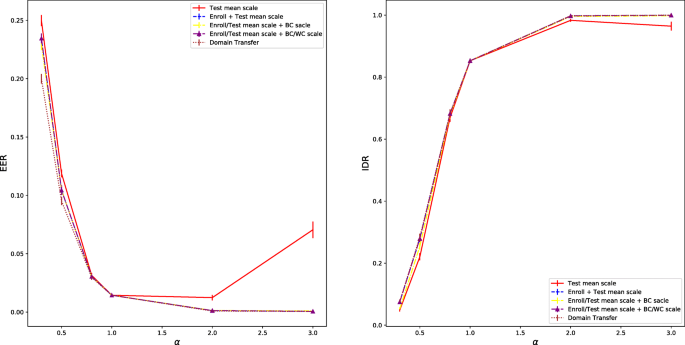

  

  Performance loss with the class mean scale mismatch between enrollment and test. The x-axis represents the scale factor α

• Blue curve: Scale the enrollment data and the class means of the test data in the same way, and use the between-class and within-class variances of the original enrollment data when computing the NL score. Since the enrollment data is scaled, the mean mismatch problem is solved, however the between-class distribution mismatch remains.

• Yellow curve: Scale the enrollment data and the class means of the test data in the same, and use the between-class variance of the scaled enrollment data (that is correct for both enrollment and test) and the within-class variance of the original enrollment data (that is correct for test but incorrect for enrollment) when computing the NL score. This approach solves the mean mismatch and between-class distribution mismatch, but the within-class variance is incorrect for enrollment.

• Purple curve: Scale the enrollment data and the class means of the test data in the same way, and use the between-class variance of the scaled enrollment data (that is correct for both enrollment and test) and the within-class variance of the scaled enrollment data (that is correct for enrollment but incorrect for test) when computing the NL score. This approach solves the mean mismatch and between-class distribution mismatch, but the within-class variance is incorrect for test.

• Brown curve: Apply condition transfer that will be presented shortly.

From Fig. 13, it can be seen that scaling the class means of the test data caused serious performance reduction, especially when the scale is large. Scaling the enrollment data to match the test data seems can mitigate this problem to a large extent. The impact of using the incorrect between-class and within-class distributions is not very substantial, indicating that mean mismatch is more serious compared to distribution mismatch in NL scoring. Finally, the condition transfer approach obtains the best performance, by correcting both the mean mismatch and the distribution mismatch.

3.6.3 Mean shift

In the third experiment, we shift the class means by β on each dimension when sampling the test data. This mean shift causes two problems for NL scoring: (1) mean mismatch: the class means of the enrollment data do not match the class means of the test data, leading to incorrect likelihood p_k(x|μ), thus incorrect p_k(x); (2) between-class distribution shift: the between-class distribution of the test data is shifted in the same way as the mean shift, which leads to incorrect normalization p(x).

A simple compensation is to shift the enrollment data in the same way as the test data. After the shift, the mean mismatch problem is mitigated, however the NL still uses the between-class distribution of the original enrollment data. This is essentially the data shift scenario in the domain mismatch experiment. Another compensation is to compute the posterior of the class mean p(μ|x) first, and then shift the mean of the posterior in the same way as the test data. By this way, the mean mismatch is solved and the likelihood p_k(x) is correct; however, the normalization p(x) is incorrect due to the shifted between-class distribution of the test data.

We report the results of four tests in Fig. 14:

• Red curve: Shift the test data only. This is the case with no compensation.

  Fig. 14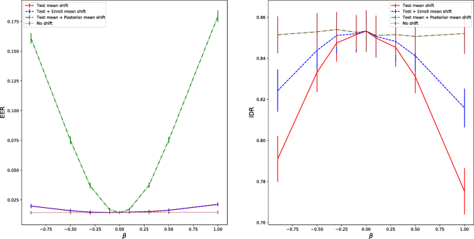

  

  Performance loss with the class mean shift between enrollment and test. The x-axis represents the value of mean shift. Note that the green curve is overlapped by the brown curve in the IDR plot

• Blue curve: Shift the enrollment and test data in the same way. This is the data shift scenario in the domain mismatch experiment.

• Green curve: Shift the test data, and then shift the mean of the posterior p(μ|x). It fully solves the mean mismatch problem; however, the normalization p(x) is incorrect due to the shifted between-class distribution.

• Brown curve: No data shift.

The results shown in Fig. 14 demonstrate that the mean shift on test data tends to cause significant performance degradation (red curve vs brown curve). This loss is comparable or even worse compared to the domain mismatch case (red curve vs blue curve). If we remove the mean mismatch but uses the incorrect normalization (green curve), the IDR performance recovers perfectly but the EER results become worse. The good performance on IDR is expected as the normalization term does not impact decisions of the SI task. The bad performance on EER demonstrates that an incorrect normalization may cause fatal performance loss on the SV task. An interesting observation is that for the EER results, removing the mean mismatch makes the performance even worse compared to doing nothing (green curve vs. red curve). This suggests that the errors caused by mean mismatch and between-class distribution shift are in opposite directions.

3.7 Condition transfer

We present a simple condition transfer approach based on the NL scoring, which is optimal under the linear Gaussian assumption. For simplicity, we will assume that the data have been shifted appropriately, so that the mean-shift problem does not exist. Denote the parameters of the NL models suitable for the enrollment and test data by {ε,σ} and $\left \{\hat {\boldsymbol {\epsilon }}, \hat {\boldsymbol {\sigma }}\right \}$ respectively. Note that we have allowed a non-isotropic within-class covariance $\mathbf {I}\hat {\boldsymbol {\sigma }}^{2}$ for the test data. Given enrollment samples $\boldsymbol {x}^{k}_{1},...\boldsymbol {x}^{k}_{n_{k}}$ of class k, the posterior of its class mean will be computed using the between-class and within-class variances of the enrollment data:

$$ {}p\left(\boldsymbol{\mu}_{k} |\boldsymbol{x}^{k}_{1},...\boldsymbol{x}^{k}_{n_{k}} \right) = N\left(\boldsymbol{\mu}_{k} ; \frac{n_{k} \boldsymbol{\epsilon}^{2}}{n_{k} \boldsymbol{\epsilon}^{2} + \sigma^{2}} \bar{\boldsymbol{x}}_{k}, \mathbf{I} \frac{\boldsymbol{\epsilon}^{2} \sigma^{2}}{n_{k} \boldsymbol{\epsilon}^{2} + \sigma^{2}} \right). $$

(40)

Since there is no data shift, this posterior can be readily used to estimate the likelihood of the test sample, using the within-class variance $\hat {\boldsymbol {\sigma }}$ of the test data:

$$ p_{k}(\boldsymbol{x}) = N\left(\boldsymbol{x} ; \frac{n_{k} \boldsymbol{\epsilon}^{2}}{n_{k} \boldsymbol{\epsilon}^{2} + \sigma^{2}} \bar{\boldsymbol{x}}_{k}, \mathbf{I} \left(\hat{\boldsymbol{\sigma}}^{2} + \frac{\boldsymbol{\epsilon}^{2} \sigma^{2}}{n_{k} \boldsymbol{\epsilon}^{2} + \sigma^{2}}\right) \right). $$

(41)

Augmented by the normalization term computed using the between-class and within-class variances of the test data, the NL score will have the following form:

$$ \log NL (\boldsymbol{x} |k) \propto -\left\|\frac{\boldsymbol{x} - \tilde{\boldsymbol{\mu}}_{k}}{ \sqrt{\hat{\boldsymbol{\sigma}}^{2} + \frac{\boldsymbol{\epsilon}^{2} \sigma^{2}}{n_{k} \boldsymbol{\epsilon}^{2} + \sigma^{2}}}} \right\|^{2} + \left\|\frac{\boldsymbol{x}}{\hat{\boldsymbol{\epsilon}}^{2} + \hat{\boldsymbol{\sigma}}^{2}} \right\|^{2}, $$

(42)

where

$$ \tilde{\boldsymbol{\mu}}_{k} = \frac{n_{k} \boldsymbol{\epsilon}^{2}}{n_{k} \boldsymbol{\epsilon}^{2} + \sigma^{2}} \bar{\boldsymbol{x}}_{k}. $$

(43)

The condition transfer approach described above can be easily extended to handel more complex condition mismatch, which will be left for future work. Note that we have shown the performance of this method in Figs. 12 and 13. In both cases, it provides the best (actually optimal) performance.

4 Discussion

The NL formulation plays a central role in our simulation study. From the perspective of NL scoring, any performance loss can be attributed to data-model mismatch on the three components of the NL scoring: the enrollment model $p\left (\boldsymbol {\mu }|\boldsymbol {x}_{1},..., \boldsymbol {x}_{n_{k}}\right)$, the prediction model p(x|μ), and the normalization model p(x). The mismatch could be (1) mismatch on distribution type (e.g., Gaussian assumed but Laplacian in reality), (2) mismatch on the mean (mean mismatch), and (3) mismatch on the covariance (covariance mismatch). This analytical view provides a powerful and necessary tool for our simulation study. By this tool, we can analyze how a particular imperfection causes performance reduction, and design suitable algorithms to compensate for the impact, e.g., the conditional transfer algorithm.

The simulation results show that for a practical speaker recognition system, mean mismatch is the most risky. For example, in the data shift scenario of the domain mismatch experiment, the mean of the between-class distribution does not match the data, causing between-class mean mismatch; in the mean shift scenario of the enrollment-test condition mismatch experiment, the means of the within-class distributions of individual classes do not match the data, causing within-class mean mismatch. The performance reduction on these two scenarios is much more significant compared to on other scenarios.

Although our work focuses on the linear Gaussian NL, the NL formulation is general and can be easily extended by using nonlinear and non-Gaussian models, so that it deal with more complex data. Recently, we provide such an extension [64], by applying the invariance property of the NL score under invertible transforms, as discussed in Section 2.3. Specifically, we learn an invertible transform that maps the original data to a latent space where the data can be modeled by a linear Gaussian. According to the equivalence of the NL score in the original and the transformed space, this transform allows us using a linear Gaussian NL model to score data with a complex distribution. This is essentially a nonlinear extension of the PLDA model, which we call neural discriminant analysis (NDA). In our previous study, the NDA model produces very promising results [64].

The MBR optimum of the NL scoring may encourage more research on the speaker embedding approach. Since we have known that the NL score is MBR optimal, its performance will be ensured if the distribution of the speaker vectors meet the assumption of the model. This performance insurance represents a clear advantage of the embedding approach compared to the so-called end-to-end approach [65–67]. Moreover, since the NL score is optimal if and only if the speaker vectors follow the assumed generative model, more research is encouraged on normalizing the speaker vectors, rather than pursuing other complicated scoring methods (e.g., discriminative PLDA [68]) or score calibration [69, 70]. Our recent work shows that speaker vector normalization is highly promising [50].

Finally, the main purpose of the paper is a full understanding for the NL score by simulation, so we have refrained from presenting any EER/IDR results on real SRE systems (large-scale experiments for the NL score with real data have been presented by other papers, e.g., [64]). We found that the simulation study is very useful and offers a lower bound and an upper bound for a potential technique. For the lower bound, it gives a clear justification that a technique does work if the presumed condition is matched, and so what we should do is to meet the condition. For the upper bound, it tells the maximum that a technique can achieve if the presumed condition is perfectly matched, so we should not intend to seek for more in real applications.

5 Conclusions

We present an analysis on the optimal score for speaker recognition based on the MAP principle and the linear Gaussian assumption. The analysis shows that the normalized likelihood (NL) is optimal for both identification and verification tasks in the sense of minimum Bayes risk. We also show that the NL score based on the linear Gaussian model is equivalent to the popular PLDA LR. The cosine score and Euclidean score can be regarded as two approximations of the optimal NL score. Comprehensive simulation experiments were conducted to study the behavior of the NL score, especially at the operation point of a true speaker recognition system. The major knowledge we obtained from the simulation study is that the NL performance may be seriously reduced by real-life imperfections, including the non-Gaussianality and non-homogeneity of the data, inaccurate estimation of the between-class and within-class variances, and potential mismatch between enrollment and test conditions. Among all the detrimental factors, data shift caused the most significant performance reduction. We also proposed a condition transfer approach that can compensate for the enrollment-test mismatch.

References

J. P. Campbell, Speaker recognition: a tutorial. Proc. IEEE. 85(9), 1437–1462 (1997).
D. A. Reynolds, in IEEE International Conference on Acoustics, Speech, and Signal Processing (ICASSP). An overview of automatic speaker recognition technology, (2002), pp. 4072–4075.
J. H. Hansen, T. Hasan, Speaker recognition by machines and humans: a tutorial review. IEEE Signal Proc. Mag.32(6), 74–99 (2015).
N. Dehak, P. J. Kenny, R. Dehak, P. Dumouchel, P. Ouellet, Front-end factor analysis for speaker verification. IEEE Trans. Audio Speech Lang. Process.19(4), 788–798 (2011).
E. Variani, X. Lei, E. McDermott, I. L. Moreno, J. Gonzalez-Dominguez, in IEEE International Conference on Acoustics, Speech and Signal Processing (ICASSP). Deep neural networks for small footprint text-dependent speaker verification, (2014), pp. 4052–4056.
L. Li, Y. Chen, Y. Shi, Z. Tang, D. Wang, in Proceedings of the Annual Conference of International Speech Communication Association (INTERSPEECH). Deep speaker feature learning for text-independent speaker verification, (2017), pp. 1542–1546.
J. S. Chung, A. Nagrani, A. Zisserman, in Proceedings of the Annual Conference of International Speech Communication Association (INTERSPEECH). VoxCeleb2: deep speaker recognition, (2018), pp. 1086–1090.
J. -W. Jung, H. S. Heo, J. -H. Kim, H. -J. Shim, H. -J. Yu, in Proceedings of the Annual Conference of International Speech Communication Association (INTERSPEECH). RawNet: advanced end-to-end deep neural network using raw waveforms for text-independent speaker verification, (2019), pp. 1268–1272.
K. Okabe, T. Koshinaka, K. Shinoda, in Proceedings of the Annual Conference of International Speech Communication Association (INTERSPEECH). Attentive statistics pooling for deep speaker embedding, (2018), pp. 2252–2256.
W. Cai, J. Chen, M. Li, in Proceedings of Odyssey: The Speaker and Language Recognition Workshop. Exploring the encoding layer and loss function in end-to-end speaker and language recognition system, (2018), pp. 74–81.
W. Xie, A. Nagrani, J. S. Chung, A. Zisserman, in IEEE International Conference on Acoustics, Speech and Signal Processing (ICASSP). Utterance-level aggregation for speaker recognition in the wild, (2019), pp. 5791–5795.
N. Chen, J. Villalba, N. Dehak, in Proceedings of the Annual Conference of International Speech Communication Association (INTERSPEECH). Tied mixture of factor analyzers layer to combine frame level representations in neural speaker embeddings, (2019), pp. 2948–2952.
L. Li, D. Wang, C. Xing, T. F. Zheng, in 10th International Symposium on Chinese Spoken Language Processing (ISCSLP). Max-margin metric learning for speaker recognition, (2016), pp. 1–4.
W. Ding, L. He, in Proceedings of the Annual Conference of International Speech Communication Association (INTERSPEECH). MTGAN: speaker verification through multitasking triplet generative adversarial networks, (2018), pp. 3633–3637.
J. Wang, K. -C. Wang, M. T. Law, F. Rudzicz, M. Brudno1, in International Conference on Acoustics, Speech and Signal Processing (ICASSP). Centroid-based deep metric learning for speaker recognition, (2019), pp. 3652–3656.
Z. Bai, X. -L. Zhang, J. Chen, Partial AUC optimization based deep speaker embeddings with class-center learning for text-independent speaker verification. Int. Conf. Acoust. Speech Signal Process. (ICASSP), 6819–6823 (2020).
Z. Gao, Y. Song, I. McLoughlin, P. Li, Y. Jiang, L. -R. Dai, in Proceedings of the Annual Conference of International Speech Communication Association (INTERSPEECH). Improving aggregation and loss function for better embedding learning in end-to-end speaker verification system, (2019), pp. 361–365.
J. Zhou, T. Jiang, Z. Li, L. Li, Q. Hong, in Proceedings of the Annual Conference of International Speech Communication Association (INTERSPEECH). Deep speaker embedding extraction with channel-wise feature responses and additive supervision softmax loss function, (2019), pp. 2883–2887.
R. Li, N. L. D. Tuo, M. Yu, D. Su, D. Yu, in IEEE International Conference on Acoustics, Speech and Signal Processing (ICASSP). Boundary discriminative large margin cosine loss for text-independent speaker verificationIEEE, (2019), pp. 6321–6325.
S. Wang, J. Rohdin, L. Burget, O. Plchot, Y. Qian, K. Yu, J. Cernocky, in Proceedings of the Annual Conference of International Speech Communication Association (INTERSPEECH). On the usage of phonetic information for text-independent speaker embedding extraction, (2019), pp. 1148–1152.
T. Stafylakis, J. Rohdin, O. Plchot, P. Mizera, L. Burget, in Proceedings of the Annual Conference of International Speech Communication Association (INTERSPEECH). Self-supervised speaker embeddings, (2019), pp. 2863–2867.
S. O. Sadjadi, C. Greenberg, E. Singer, D. Reynolds, L. Mason, J. Hernandez-Cordero, in Proceedings of the Annual Conference of International Speech Communication Association (INTERSPEECH). The 2018 NIST Speaker Recognition Evaluation, (2019), pp. 1483–1487.
D. Snyder, D. Garcia-Romero, G. Sell, D. Povey, S. Khudanpur, in IEEE International Conference on Acoustics, Speech and Signal Processing (ICASSP). X-vectors: robust DNN embeddings for speaker recognitionIEEE, (2018), pp. 5329–5333.
S. Ioffe, in European Conference on Computer Vision (ECCV). Probabilistic linear discriminant analysisSpringer, (2006), pp. 531–542.
S. J. Prince, J. H. Elder, in 2007 IEEE 11th International Conference on Computer Vision. Probabilistic linear discriminant analysis for inferences about identityIEEE, (2007), pp. 1–8.
D. A. Reynolds, T. F. Quatieri, R. B. Dunn, Speaker verification using adapted Gaussian mixture models. Digit. Signal Proc.10(1-3), 19–41 (2000).
B. J. Borgström, A. McCree, in 2013 IEEE International Conference on Acoustics, Speech and Signal Processing. Discriminatively trained Bayesian speaker comparison of i-vectorsIEEE, (2013), pp. 7659–7662.
A. McCree, G. Sell, D. Garcia-Romero, in INTERSPEECH. Extended variability modeling and unsupervised adaptation for PLDA speaker recognition, (2017), pp. 1552–1556.
C. M. Bishop, Pattern recognition and machine learning (Springer, 2006). https://www.springer.com/gp/book/9780387310732.
A. Blum, J. Hopcroft, R. Kannan, Foundations of data science (Cambridge University Press, 2015). http://www.cs.cornell.edu/jeh/bookmay2015.pdf.
D. Garcia-Romero, C. Y. Espy-Wilson, in Proceedings of the Annual Conference of International Speech Communication Association (INTERSPEECH). Analysis of i-vector length normalization in speaker recognition systems, (2011), pp. 249–252.
W. Rudin, Real and complex analysis, 3rd Ed (McGraw-Hill, 1986). https://www.amazon.com/Real-Complex-Analysis-Higher-Mathematics/dp/0070542341.
G. Salton, Automatic text processing: The transformation, analysis, and retrieval of information by computer (Addison-Wesley, 1989). https://books.google.co.jp/books/about/Automatic_Text_Processing.html?id=wb8SAQAAMAAJ&redir_esc=y.
G. G. Chowdhury, Introduction to modern information retrieval, 3rd Ed (Neal-Schuman Publishers, 2010). https://www.amazon.com/Introduction-Modern-Information-Retrieval-3rd/dp/1555707157.
C. Xing, D. Wang, C. Liu, Y. Lin, in Proceedings of the 2015 Conference of the North American Chapter of the Association for Computational Linguistics: Human Language Technologies. Normalized word embedding and orthogonal transform for bilingual word translation, (2015), pp. 1006–1011.
N. Dehak, R. Dehak, P. Kenny, N. Brümmer, P. Ouellet, P. Dumouchel, in Proceedings of the Annual Conference of International Speech Communication Association (INTERSPEECH). Support vector machines versus fast scoring in the low-dimensional total variability space for speaker verification, (2009), pp. 1559–1562.
P. Kenny, in Proceedings of Odyssey: The Speaker and Language Recognition Workshop. Bayesian speaker verification with heavy-tailed priors, (2010), pp. 14–14. https://www.isca-speech.org/archive_open/odyssey_2010/od10_014.html.
S. Sra, Directional statistics in machine learning: a brief review. Appl. Directional Stat. Mod. Methods Case Stud., 225 (2018).
K. V. Mardia, P. E. Jupp, Directional statistics (John Wiley & Sons, Inc, 2009). https://onlinelibrary.wiley.com/doi/book/10.1002/9780470316979.
A. Nagrani, J. S. Chung, A. Zisserman, in Proceedings of the Annual Conference of International Speech Communication Association (INTERSPEECH). VoxCeleb: a large-scale speaker identification dataset, (2017), pp. 2616–2620.
D. Snyder, G. Chen, D. Povey, Musan: a music, speech, and noise corpus. arXiv preprint arXiv:1510.08484 (2015). http://arxiv.org/abs/1510.08484.
T. Ko, V. Peddinti, D. Povey, M. L. Seltzer, S. Khudanpur, in IEEE International Conference on Acoustics, Speech and Signal Processing (ICASSP). A study on data augmentation of reverberant speech for robust speech recognitionIEEE, (2017), pp. 5220–5224.
D. Povey, A. Ghoshal, G. Boulianne, L. Burget, O. Glembek, N. Goel, M. Hannemann, P. Motlicek, Y. Qian, P. Schwarz, et al., in IEEE workshop on automatic speech recognition and understanding. The Kaldi speech recognition toolkit, (2011). https://infoscience.epfl.ch/record/192584.
S. Lyu, E. P. Simoncelli, Nonlinear extraction of independent components of natural images using radial gaussianization. Neural Comput.21(6), 1485–1519 (2009).
L. Li, Z. Tang, D. Wang, T. F. Zheng, in IEEE International Conference on Acoustics, Speech and Signal Processing (ICASSP). Full-info training for deep speaker feature learningIEEE, (2018), pp. 5369–5373.
L. Li, Z. Tang, Y. Shi, D. Wang, in IEEE International Conference on Acoustics, Speech and Signal Processing (ICASSP). Gaussian-constrained training for speaker verificationIEEE, (2019), pp. 6036–6040.
Y. Zhang, L. Li, D. Wang, in Proceedings of the Annual Conference of International Speech Communication Association (INTERSPEECH). VAE-based regularization for deep speaker embedding, (2019), pp. 4020–4024.
X. Wang, L. Li, D. Wang, in Proceedings of APSIPA ASC. VAE-based Domain Adaptation for Speaker Verification, (2019), pp. 535–539.
Y. Tu, M. -W. Mak, J. -T. Chien, in Proceedings of the Annual Conference of International Speech Communication Association (INTERSPEECH). Variational domain adversarial learning for speaker verification, (2019), pp. 4315–4319.
Y. Cai, L. Li, D. Wang, A. Abel, Deep normalization for speaker vectors. arXiv:2004.04095 (2020). https://arxiv.org/pdf/2004.04095.pdf.
L. Dinh, D. Krueger, Y. Bengio, in ICLR Workshop. NICE: Non-linear independent components estimation, (2015). https://iclr.cc/archive/www/doku.php%3Fid=iclr2015:main.html.
L. Dinh, J. Sohl-Dickstein, S. Bengio, in Neural Information Processing Systems - Deep Learning Symposium. Density estimation using real NVP, (2016).
D. P. Kingma, P. Dhariwal, in Advances in Neural Information Processing Systems (NIPS). Glow: generative flow with invertible 1x1 convolutions, (2018), pp. 10215–10224.
Y. Fan, J. Kang, L. Li, K. Li, H. Chen, S. Cheng, P. Zhang, Z. Zhou, Y. Cai, D. Wang, in IEEE International Conference on Acoustics, Speech and Signal Processing (ICASSP). CN-CELEB: a challenging Chinese speaker recognition dataset, (2020), pp. 7604–7608.
H. Aronowitz, in IEEE International Conference on Acoustics, Speech and Signal Processing (ICASSP). Inter dataset variability compensation for speaker recognition, (2014), pp. 4002–4006.
J. Villalba, E. Lleida, in Proceedings of Odyssey: The Speaker and Language Recognition Workshop. Bayesian adaptation of PLDA based speaker recognition to domains with scarce development data, (2012), pp. 47–54.
D. Garcia-Romero, A. McCree, in IEEE International Conference on Acoustics, Speech and Signal Processing (ICASSP). Supervised domain adaptation for i-vector based speaker recognition, (2014), pp. 4047–4051.
D. Garcia-Romero, A. McCree, S. Shum, C. Vaquero, in Proceedings of Odyssey: The Speaker and Language Recognition Workshop. Unsupervised domain adaptation for i-vector speaker recognition, (2014), pp. 260–264.
H. Aronowitz, in Proceedings of Odyssey: The Speaker and Language Recognition Workshop. Compensating inter-dataset variability in PLDA hyper-parameters for robust speaker recognition, (2014), pp. 280–286.
A. Kanagasundaram, D. Dean, S. Sridharan, in IEEE International Conference on Acoustics, Speech and Signal Processing (ICASSP). Improving out-domain PLDA speaker verification using unsupervised inter-dataset variability compensation approach, (2015), pp. 4654–4658.
M. H. Rahman, A. Kanagasundaram, I. Himawan, D. Dean, S. Sridharan, Improving PLDA speaker verification performance using domain mismatch compensation techniques. Comput. Speech Lang.47:, 240–258 (2018).
S. Shon, S. Mun, W. Kim, H. Ko, in Proceedings of the Annual Conference of International Speech Communication Association (INTERSPEECH). Autoencoder based domain adaptation for speaker recognition under insufficient channel information, (2017), pp. 1014–1018.
Q. Wang, W. Rao, S. Sun, L. Xie, E. S. Chng, H. Li, in IEEE International Conference on Acoustics, Speech and Signal Processing (ICASSP). Unsupervised domain adaptation via domain adversarial training for speaker recognition, (2018), pp. 4889–4893.
L. Li, D. Wang, T. F. Zheng, in Interspeech 2020. Neural discriminant analysis for speaker recognition, (2020).
G. Heigold, I. Moreno, S. Bengio, N. Shazeer, in IEEE International Conference on Acoustics, Speech and Signal Processing (ICASSP). End-to-end text-dependent speaker verificationIEEE, (2016), pp. 5115–5119.
S. -X. Zhang, Z. Chen, Y. Zhao, J. Li, Y. Gong, in Spoken Language Technology Workshop (SLT). End-to-end attention based text-dependent speaker verificationIEEE, (2016), pp. 171–178.
F. R. rahman Chowdhury, Q. Wang, I. L. Moreno, L. Wan, in IEEE International Conference on Acoustics, Speech and Signal Processing (ICASSP). Attention-based models for text-dependent speaker verification, (2018), pp. 5359–5363.
L. Burget, O. Plchot, S. Cumani, O. Glembek, P. Matějka, N. Brümmer, in IEEE International Conference on Acoustics, Speech and Signal Processing (ICASSP). Discriminatively trained probabilistic linear discriminant analysis for speaker verificationIEEE, (2011), pp. 4832–4835.
D. A. Van Leeuwen, N. Br, in Proceedings of the Annual Conference of International Speech Communication Association (INTERSPEECH). The distribution of calibrated likelihood-ratios in speaker recognition, (2013), pp. 1619–1623.
S. Cumani, P. Laface, in IEEE International Conference on Acoustics, Speech and Signal Processing (ICASSP). Tied normal variance - mean mixtures for linear score calibration, (2019), pp. 6121–6125.
Acknowledgements
Thanks to Dr. Lantian Li, Yunqi Cai, and Zhiyuan Tang for the valuable discussion.
Funding
This work was supported by the National Natural Science Foundation of China (NSFC) under the project No.61633013 and No.61371136.
Author information
Authors and Affiliations
Contributions
All the work was completed by DW. The author read and approved the final manuscript.
Corresponding author
Ethics declarations
Competing interests
The authors declare that they have no competing interests.
Additional information
Publisher’s Note
Springer Nature remains neutral with regard to jurisdictional claims in published maps and institutional affiliations.
Rights and permissions
Open Access This article is licensed under a Creative Commons Attribution 4.0 International License, which permits use, sharing, adaptation, distribution and reproduction in any medium or format, as long as you give appropriate credit to the original author(s) and the source, provide a link to the Creative Commons licence, and indicate if changes were made. The images or other third party material in this article are included in the article’s Creative Commons licence, unless indicated otherwise in a credit line to the material. If material is not included in the article’s Creative Commons licence and your intended use is not permitted by statutory regulation or exceeds the permitted use, you will need to obtain permission directly from the copyright holder. To view a copy of this licence, visit http://creativecommons.org/licenses/by/4.0/.
About this article
Cite this article
Wang, D. A simulation study on optimal scores for speaker recognition. J AUDIO SPEECH MUSIC PROC. 2020, 18 (2020). https://doi.org/10.1186/s13636-020-00183-3
Received:
Accepted:
Published:
DOI: https://doi.org/10.1186/s13636-020-00183-3