Steerable differential beamformers with planar microphone arrays

Abstract

Humanoid robots require to use microphone arrays to acquire speech signals from the human communication partner while suppressing noise, reverberation, and interferences. Unlike many other applications, microphone arrays in humanoid robots have to face the restrictions in size and geometry. To address these challenges, this paper presents an approach to differential beamforming with arbitrary planar array geometries. The major contributions of this work are as follows: (1) a method is presented to design differential beamformers, which works for regular geometries such as linear, circular, and concentric circular ones, as well as irregular geometries, as long as the sensors’ positions are given or can be measured; (2) fundamental requirements for the design of different orders of linear differential microphone arrays (DMAs), partially steerable DMAs, fully steerable DMAs, and robust DMAs are discussed; (3) the validity and limitations of the Jacobi-Anger expansion approximation is analyzed, where we discuss how to achieve an optimal approximation by properly choosing the reference point; and (4) we show how to design an Nth-order DMA with 2N microphones using the Jacobi-Anger expansion.

1 Introduction

It has long been a dream of researchers and engineers to create humanoid robots, which can communicate naturally with humans through speech and language. A prerequisite for this is the ability to acquire speech from the human communication partner with high fidelity/quality and, meanwhile, mitigate or even eliminate the effects of background noise, acoustic feedback, interferences, reverberation, and robot ego noise. This requires to use sensor arrays with multiple microphones arranged into a certain geometry. Unlike many well-studied applications such as teleconferencing, microphone arrays for robot audition are limited by size and geometry [1–5]. Therefore, how to design small arrays with a flexible geometry and the associated beamforming algorithms that can process broadband speech signals is a critical problem [6–13]. Among different types of available arrays, differential microphone arrays (DMAs), which are designed to measure the differentials of the sound pressure field, are more appropriate for robot audition since they are small in size and can achieve high directivity and frequency-invariant beampatterns [14–23]. From the early efforts of designing linear DMAs in a multistage manner [24, 25], to the recently developed null-constraint-based linear DMAs in the short-time Fourier transform (STFT) domain [26], the flexibility in forming different beampatterns and the robustness of differential beamformers have been significantly improved [27–31].

An important issue in applications of DMAs is the steering flexibility. Linear DMAs do not have much flexibility in terms of beam steering: the beampattern varies with the steering angle and the optimal performance in terms of directivity factor (DF) occurs only at the endfire directions, i.e., the directions along the line that connects all sensors [26, 32]. A number of efforts have been devoted to improving the steering flexibility of DMAs. In [33, 34], two-dimensional arrays are used to form multiple linear DMAs, and the resulting beampatterns can be steered to a certain number of directions. In [35, 36], first-order steerable DMAs were constructed by a linear combination of monopole and two orthogonal dipoles using a four-element square array. In [37], uniform circular DMAs (CDMAs) were designed and their beampatterns can be perfectly steered to M different directions, i.e., the M angular positions of the array elements. In [38], the authors proposed a steerable second-order DMA as a linear combination of a monopole and dipoles with seven or nine microphones. In [39], a method was proposed to design a nearly constant beampattern, which can be continuously steered between two directions of the reference beams. In [40], an approach was developed to the design of CDMAs based on an approximation of the beampattern from a least-squares error (LSE) perspective, where the designed beampattern is almost frequency invariant and can be steered to any look direction in the sensor plane. In [41], concentric circular DMAs (CCDMAs) were developed, which can achieve full flexibility in beam steering in the sensor’s plane and have a flexible array structure (a smaller ring can have less microphones than a larger one).

While great progress has been achieved in the design of DMAs with high directivity, frequency-invariant beampatterns, high robustness, and good steering flexibility, only a few efforts can be found in the literature to deal with flexibility in array geometry. In [42, 43], a method was presented to design a frequency-invariant beamformer based on spherical harmonic decompositions. While it is adaptable to an arbitrary array and it is steerable, the solution does not guarantee a perfectly frequency-invariant beampattern. In [44], a broadband beamformer was proposed for spherical arrays with arbitrary sensor configurations, where the sensors’ positions do not have to satisfy the orthonormality criterion, but the shape of the array is limited to spherical. In [45], a general model was developed to design superdirective beamformers for arbitrary sensor arrays. In [46], the authors extended the work in [43] to develop a steerable beamformer for arbitrary planar arrays, but the beampatterns are not frequency invariant. While they have led to many interesting results, the aforementioned efforts did not address the general problem of differential beamforming. Therefore, further efforts are indispensable to study how to design differential beamformers with flexibility in sensor configurations.

In a recent work [7], we studied the problem of differential beamforming with microphone arrays of arbitrary planar geometry, but many important issues such as beampattern steering, influence of array geometry on beamforming performance, and requirements for designing different beampatterns were not addressed. This work is basically an extension of the study in [7]. In comparison with [7], the major contributions of this paper are as follows. First, a detailed analysis is presented on the design of DMAs to address such issues as the basic requirements for the design of different orders of linear DMAs (LDMAs), limited steerable DMAs (LSDMAs), continuously steerable DMAs (CSDMAs), and robust DMAs. Second, we discuss the validity and limitations of the Jacobi-Anger expansion approximation, where we propose to achieve an optimal approximation with fixed array geometry and number of microphones by choosing an appropriate reference. Generally, the value of r_m, i.e., the distance from the reference point to the mth sensor, determines the accuracy of the approximation. Consequently, with fixed array geometry and number of microphones, we can improve DMAs performance by choosing appropriate reference points, i.e., making the value of r_m as small as possible. Third, we present the case of designing an Nth-order DMA with 2N microphones. In previous studies of designing differential beamformers with Jacobi-Anger expansion, at least 2N+1 microphones are needed to design an Nth-order DMAs. We prove that with the Jacobi-Anger expansion, we can also design an Nth-order DMA with 2N microphones, but the designed beampattern can be only perfectly steered to M different directions, i.e., the angular positions of the M array elements. This is consistent with the previous conclusion of null-constraint circular differential microphone arrays [37].

The organization of this paper is as follows. Section 2 presents the signal model, problem formulation, and performance measures. Section 3 describes the desired target frequency-invariant beampattern. Section 4 discusses how to design differential beamformers with arbitrary array geometries and presents some special cases. Section 5 demonstrates the design of first-, second-, and third-order DMAs and analyzes the steering flexibility. Section 6 presents some simulation results to validate the theoretical derivations, and conclusions are given in Section 7.

2 Signal model, problem formulation, and performance measures

We consider an array consisting of M sensors, which are distributed in a specified area on a plane. Assume that the center of the array coincides with the origin of the two-dimensional Cartesian coordinate system and the azimuthal angles are measured anti-clockwise from the x axis. The coordinates of the microphones are then written as r_m=r_m[cosψ_m sinψ_m]^T, with m=1,2,…,M, where the superscript ^T is the transpose operator, r_m is the distance from the mth microphone to the origin point, and ψ_m is the angular position of the mth array element. The distance between microphones i and j (for i,j=1,2,…,M) is then

$$\begin{array}{*{20}l} \delta_{ij} = \left \| \mathbf{r}_{i} - \mathbf{r}_{j} \right \|_{2}, \end{array} $$

(1)

where ∥·∥₂ denotes the Euclidean norm. In this paper, we consider small-size arrays and assume that δ_max≪λ_min, where δ_max= max{δ_ij, i,j=1,2,…,M}, with λ_min being the smallest acoustic wavelength in the frequency band of interest. This assumption ensures that the true acoustic pressure differentials can be approximated by finite differences between the microphones’ outputs in the design of DMAs.

With the small spacing assumption, it is natural to consider the farfield scenario. Assume that the incidence angle is characterized by azimuthal angle θ. If we define the wavenumber as k=−(ω/c)[cosθ sinθ]^T, the steering vector of length M corresponding to the array is written as [47]

$$\begin{array}{*{20}l} \mathbf{d}\left(\omega,\theta \right) &= \left[ \begin{array}{ccc} e^{-\jmath \mathbf{k}^{T} \mathbf{r}_{1}} & \cdots & e^{-\jmath \mathbf{k}^{T} \mathbf{r}_{M}} \end{array} \right]^{T} \\ &= \left[ e^{\jmath\omega r_{1} \cos\left(\theta - \psi_{1} \right)/c} ~~ \cdots ~~ e^{\jmath\omega r_{M} \cos\left(\theta - \psi_{M} \right)/c} \right]^{T}, \end{array} $$

(2)

where ȷ is the imaginary unit, ω=2πf is the angular frequency, and f>0 is the temporal frequency.

The objective of beamforming is to recover the source signal of interest that is corrupted by spatial acoustic noise. For that, the signal received at each microphone is multiplied by a complex weight, $H_{m}^{*} \left (\omega \right), \ m=1,2,\ldots,M$, where the superscript ^∗ stands for complex conjugation. The weighted outputs are then summed together to form the beamformer’s output [8]. Stacking all the weights together in a vector of length M, we get

$$\begin{array}{*{20}l} \mathbf{h}(\omega) = \setlength\arraycolsep{2pt} \left[ \begin{array}{cccc} H_{1} \left(\omega \right) & H_{2} \left(\omega \right) & \cdots & H_{M} \left(\omega \right) \end{array} \right]^{T}. \end{array} $$

(3)

Without loss of generality, the distortionless constraint at the look direction (where the desired source is located, θ_s) is desired, i.e.,

$$\begin{array}{@{}rcl@{}} \mathbf{h}^{H}(\omega) \mathbf{d}\left(\omega,\theta_{\mathrm{s}} \right) =1, \end{array} $$

(4)

where the superscript ^H is the conjugate-transpose operator. Then, the problem of beamforming is to find the optimal filter with the constraint in (4) so that the beamformer’s output is a good estimate of the source signal of interest. One way of finding such a filter is by making its beampattern as close as possible to a desired target beampattern, which is the approach taken in this work.

In order to evaluate the performance of the designed beamformers, we will use the three commonly used metrics, i.e., the white noise gain (WNG), the directivity factor (DF), and the beampattern.

The WNG evaluates the robustness of a beamformer with respect to the presence of array imperfections as well as other uncertainties. It is defined as [25]

$$\begin{array}{*{20}l} {\mathcal{W}}\left[\mathbf{h}(\omega) \right] &= \frac{\left| \mathbf{h}^{H}(\omega) \mathbf{d}\left(\omega,\theta_{\mathrm{s}} \right) \right|^{2}} {\mathbf{h}^{H}(\omega) \mathbf{h}(\omega)}. \end{array} $$

(5)

The DF quantifies the ability of the beamformer in suppressing spatial noise from directions other than the look direction and it can be written as [48]

$$\begin{array}{*{20}l} {\mathcal{D}} \left[\mathbf{h}(\omega) \right] &= \frac{\left| \mathbf{h}^{H} (\omega) \mathbf{d}\left(\omega,\theta_{\mathrm{s}} \right) \right|^{2}} {\mathbf{h}^{H}(\omega) \boldsymbol{\Gamma}_{\mathrm{d}}(\omega) \mathbf{h}(\omega)}, \end{array} $$

(6)

where Γ_d(ω) is the pseudo-coherence matrix of the noise signal in a diffuse (spherically isotropic) noise field, whose (i,j)th element is

$$\begin{array}{*{20}l} \left[ \boldsymbol{\Gamma}_{\mathrm{d}}(\omega) \right]_{ij} &= \text{sinc} \left(\frac{\omega \delta_{ij}} {c} \right), \end{array} $$

(7)

with δ_ij being defined in (1).

The beampattern describes the sensitivity of the beamformer to a plane wave impinging on the array from the direction θ. Mathematically, it is defined as

$$\begin{array}{*{20}l} {\mathcal{B}} \left[ \mathbf{h}(\omega),\theta \right] &= \mathbf{h}^{H}(\omega) \mathbf{d}\left(\omega, \theta \right) \\ &= \sum_{m=1}^{M} H_{m}^{*}(\omega) e^{\jmath \omega r_{m} \cos\left(\theta - \psi_{m} \right)/c}. \end{array} $$

(8)

3 Desired target beampattern for DMAs

DMAs refer to arrays that combine closely spaced sensors to respond to the spatial derivatives of the acoustic pressure field. Early DMAs are based on the uniform linear geometry where differential beamformers are designed in a multistage manner and measure the differentials of the acoustic pressure field by combining the outputs of a number of omnidirectional sensors [25, 49]. A different DMA design method was developed in the STFT domain involves solving a system of linear equations to make the designed beampattern equal a target beampattern [26], which provides a better way to deal with white noise amplification. In this paper, we follow the framework to design differential beamformers with their beampatterns being as close as possible to a target beampattern.

Conventionally, in the design of linear DMAs, the best DF is at the endfire direction, i.e., θ=0^∘ (or 180^∘). The Nth-order frequency-invariant beampattern with its main beam pointing to the direction of 0^∘ is given by [26, 49]

$$\begin{array}{*{20}l} {\mathcal{B}} \left(\mathbf{a}_{N}, \theta \right) &= \sum_{n=0}^{N} a_{N,n} \cos \left(n \theta \right), \end{array} $$

(9)

where a_N,n, n=0,1,…,N are real-valued coefficients and

$$\begin{array}{*{20}l} \mathbf{a}_{N} &= \left[ \begin{array}{ccccc} a_{N, 0} & \cdots & a_{N,1} & \cdots & a_{N,N} \end{array} \right]^{T}. \end{array} $$

(10)

The values of the coefficients a_N,n, n=0,1,…,N in (9) affect the shape of the beampattern of the Nth-order DMA as well as its DF and WNG [25, 49]. One can determine the values of those coefficients using either the a priori information or based on some optimization criteria. For example, maximizing the directivity factor gives the hypercardioid beampattern and maximizing the front-to-back ratio leads to the supercardioid beampattern.

In the direction of the main beam, which is assumed to be θ=0^∘ for linear DMAs, the directivity pattern should be equal to 1, i.e., ${\mathcal {B}} \left (\mathbf {a}_{N}, 0^{\circ } \right) = 1$. Therefore, we have

$$\begin{array}{@{}rcl@{}} \sum_{n=0}^{N} a_{N,n} =1. \end{array} $$

(11)

In this paper, we attempt to design DMAs with arbitrary planar geometries, whose main beam is no longer limited to the direction of 0^∘. Let us assume that we want to steer the beampattern to the angle θ_s. Using the fact that cos(nθ)=(e^ȷnθ+e^−ȷnθ)/2, one can write the frequency-invariant beampattern as [40]

$$\begin{array}{*{20}l} {\mathcal{B}} \left(\mathbf{b}_{2N}, \theta-\theta_{\mathrm{s}} \right) &= \sum_{n=-N}^{N} b_{2N,n} e^{\jmath n\left(\theta-\theta_{\mathrm{s}}\right)}, \end{array} $$

(12)

where $b_{2N,0} = a_{N,0}, b_{2N,i} = \frac {1}{2} a_{N,i}, \ i=\pm 1, \ldots,\pm N$. It is more convenient to write (12) into the following vector form:

$$\begin{array}{*{20}l} {\mathcal{B}} \left(\mathbf{b}_{2N}, \theta-\theta_{\mathrm{s}} \right) &= \left[ \boldsymbol{\Upsilon}\left(\theta_{\mathrm{s}} \right) \mathbf{b}_{2N} \right]^{T} \mathbf{p}_{e}(\theta) \\ &= \mathbf{c}_{2N}^{T}\left(\theta_{\mathrm{s}} \right) \mathbf{p}_{e}(\theta) \\ &= {\mathcal{B}} \left[ \mathbf{c}_{2N}\left(\theta_{\mathrm{s}} \right), \theta \right], \end{array} $$

(13)

where

$$\begin{array}{*{20}l} \boldsymbol{\Upsilon}\left(\theta_{\mathrm{s}} \right) &= \text{diag}\left(e^{\jmath N \theta_{\mathrm{s}}}, \ldots, 1, \ldots, e^{-\jmath N \theta_{\mathrm{s}}} \right) \end{array} $$

(14)

is a (2N+1)×(2N+1) diagonal matrix and

$$\begin{array}{*{20}l} \mathbf{b}_{2N} &= \left[ \begin{array}{ccccc} b_{2N,-N} & \cdots & b_{2N,0} & \cdots & b_{2N,N} \end{array} \right]^{T}, \\ \mathbf{p}_{e}(\theta) &= \left[ \begin{array}{ccccc} e^{-\jmath N \theta} & \cdots & 1 & \cdots & e^{\jmath N \theta} \end{array} \right]^{T}, \\ \mathbf{c}_{2N}\left(\theta_{\mathrm{s}} \right) &= \boldsymbol{\Upsilon}\left(\theta_{\mathrm{s}} \right) \mathbf{b}_{2N} \\ &= \left[ c_{2N,-N}\left(\theta_{\mathrm{s}} \right) ~ \cdots ~ c_{2N,0}\left(\theta_{\mathrm{s}} \right) ~ \cdots ~ c_{2N,N}\left(\theta_{\mathrm{s}} \right) \right]^{T} \end{array} $$

are vectors of length 2N+1. Clearly, the main beam of (13) points in the direction θ_s and ${\mathcal {B}} \left [ \mathbf {c}_{2N}\left (\theta _{\mathrm {s}} \right), \theta \right ]$ is symmetric with respect to the axis θ_s ⇔ θ_s + π. The values of the coefficients of widely used beampatterns, i.e., dipole, cardioid, supercardioid, and supercardioid, are summarized in Table 1 (for the interested reader, please see [37] for the plots of those beampatterns). In this work, the beampatterns given in (13) are used as the target beampatterns to design DMAs.

Table 1 Values of the vector b_2N of the first-, second-, and third-order dipole, cardioid, supercardioid, and hypercardioid

4 Design of differential beamformers

In the design of differential beamformers with an arbitrary planar array geometry, the objective is to find a proper beamforming filter, h(ω), so that the designed beampattern, ${\mathcal {B}} \left [ \mathbf {h}(\omega),\theta \right ]$, is as close as possible to the target frequency-invariant beampattern, ${\mathcal {B}} \left [ \mathbf {c}_{2N}\left (\theta _{\mathrm {s}} \right), \theta \right ]$, i.e.,

$$\begin{array}{*{20}l} {\mathcal{B}} \left[ \mathbf{h}(\omega),\theta \right] & \approx {\mathcal{B}} \left[ \mathbf{c}_{2N}\left(\theta_{\mathrm{s}} \right), \theta \right], \ \forall \omega. \end{array} $$

(15)

In what follows, we show how to design such a beamformer.

To make ${\mathcal {B}} \left [ \mathbf {h}(\omega),\theta \right ]$ close to ${\mathcal {B}} \left [ \mathbf {c}_{2N}\left (\theta _{\mathrm {s}} \right), \theta \right ]$, we need to approximate the exponential function that appears in (8) in terms of e^ȷnθ. In our previous work in [40], we found that the optimal approximation of the exponential function that appears in beamformer’s beampattern, ${\mathcal {B}} \left [ \mathbf {h}(\omega),\theta \right ]$, from a least-squares error perspective is the Jacobi-Anger expansion [50, 51], i.e.,

$$\begin{array}{*{20}l} e^{\jmath \omega r_{m} \cos\left(\theta - \psi_{m} \right) / c} = \sum_{n=-\infty}^{\infty} \jmath^{n} J_{n} \left(\omega r_{m}/c \right) e^{\jmath n \left(\theta - \psi_{m} \right) }, \end{array} $$

(16)

where J_n(x) is the nth-order Bessel function of the first kind with J_−n(x)=(−1)ⁿJ_n(x). By limiting the expansion to the order $\pm N, {\mathcal {B}} \left [ \mathbf {h}(\omega), \theta \right ]$ can be approximated by

$$\begin{array}{*{20}l} e^{\jmath \omega r_{m} \cos\left(\theta - \psi_{m} \right) /c } \approx \sum_{n=-N}^{N} \jmath^{n} J_{n} \left(\omega r_{m}/c \right) e^{\jmath n \left(\theta - \psi_{m} \right) }. \end{array} $$

(17)

Generally, the intersensor spacing should be small enough to make the Jacobi-Anger series a good approximation of the exponential function. More precisely, the value of J_n(ωr_m/c),|n|>N determines the accuracy of the approximation. Figure 1 plots J_n(ωr_m/c) for different values of n. As seen, as ωr_m/c increases, the truncation error of higher orders increases. When ωr_m/c is large, the zeros of Bessel functions will lead to serious performance degradation [52]. With fixed array geometry and number of microphones, the reference point should be properly chosen to make the value of r_m as small as possible for an optimal approximation.

Fig. 1

The value of J_n(ωr_m/c) for different values of n

Substituting (17) into (8), we obtain

$$\begin{array}{*{20}l} {}{\mathcal{B}} \left[ \mathbf{h}(\omega),\theta \right] &= \sum_{m=1}^{M} H_{m}^{*} \left(\omega \right) \sum_{n=-N}^{N} \jmath^{n} J_{n} \left(\omega r_{m}/c \right) e^{\jmath n \left(\theta - \psi_{m} \right) } \\ &= \sum_{n=-N}^{N} e^{\jmath n \theta} \jmath^{n} \sum_{m=1}^{M} J_{n} \left(\omega r_{m}/c \right) e^{-\jmath n \psi_{m}} H_{m}^{*} \left(\omega \right) \\ &= \sum_{n=-N}^{N} e^{\jmath n \theta } \jmath^{n} {\boldsymbol{\psi}}_{n}^{T}(\omega) \mathbf{h}^{*}(\omega), \end{array} $$

(18)

where

$$\begin{array}{*{20}l} {}{\boldsymbol{\psi}}_{n} (\omega) &= \left[ J_{n} \left(\omega r_{1}/c \right)e^{-\jmath n \psi_{1}} ~~ \cdots ~~ J_{n} \left(\omega r_{M}/c \right)e^{-\jmath n \psi_{M}} \right]^{T} \end{array} $$

(19)

is a vector of length M.

Comparing (13) with (18), one can see the following relation:

$$\begin{array}{*{20}l} \jmath^{n} {\boldsymbol{\psi}}_{n}^{T}(\omega) \mathbf{h}^{*}(\omega) &= c_{2N,n}\left(\theta_{\mathrm{s}} \right), \end{array} $$

(20)

with $n=\pm 1,\pm 2,\dots,\pm N$. It follows immediately that

$$\begin{array}{@{}rcl@{}} \boldsymbol{\Psi}(\omega) \mathbf{h}(\omega) = \mathbf{c}^{*}_{2N}\left(\theta_{\mathrm{s}} \right), \end{array} $$

(21)

where

$$\begin{array}{@{}rcl@{}} \boldsymbol{\Psi}(\omega) = \left[ \begin{array}{c} \left(-\jmath \right)^{-N} {\boldsymbol{\psi}}_{-N}^{H}(\omega) \\ \vdots \\ \boldsymbol{\psi}_{0}^{H}(\omega) \\ \vdots \\ \left(-\jmath \right)^{N} \boldsymbol{\psi}_{N}^{H}(\omega) \end{array} \right] \end{array} $$

(22)

is a (2N+1)×M matrix.

Now, it is clear that the beamforming filter, h(ω), can be obtained by solving the linear system in (21). As a matter of fact, if M=2N+1, the solution of (21) is

$$\begin{array}{*{20}l} \mathbf{h} (\omega) &= \boldsymbol{\Psi}^{-1}(\omega) \mathbf{c}^{*}_{2N}\left(\theta_{\mathrm{s}} \right). \end{array} $$

(23)

But this beamformer is generally sensitive to sensors’ self noise and array imperfections at low frequencies.

To improve the robustness of the designed beamformer, we now consider the case of M>2N+1 and derive a beamforming filter by minimizing the norm of h(ω), i.e., h^H(ω)h(ω), subject to the equality constraints given in (20):

$$\begin{array}{*{20}l} \min_{\mathbf{h}(\omega)} \mathbf{h}^{H}(\omega) \mathbf{h}(\omega) ~~~\mathrm{s. \ t.} ~~~ \boldsymbol{\Psi}(\omega) \mathbf{h}(\omega) = \mathbf{c}^{*}_{2N}\left(\theta_{\mathrm{s}} \right), \end{array} $$

(24)

whose solution is

$$\begin{array}{*{20}l} \mathbf{h} (\omega) &= \boldsymbol{\Psi}^{H}(\omega) \left[ \boldsymbol{\Psi}(\omega) \boldsymbol{\Psi}^{H}(\omega) \right]^{-1} \mathbf{c}^{*}_{2N}\left(\theta_{\mathrm{s}} \right) \\ &= \boldsymbol{\Psi}^{H}(\omega) \left[ \boldsymbol{\Psi}(\omega) \boldsymbol{\Psi}^{H}(\omega) \right]^{-1} \boldsymbol{\Upsilon}^{*}\left(\theta_{\mathrm{s}} \right) \mathbf{b}_{2N}. \end{array} $$

(25)

This optimization process is equivalent to the maximization of the WNG if the array aperture is small and the approximation error in the desired direction is negligible.

A special case is when the M microphones are distributed in a uniform linear way. If the first sensor is chosen as the reference point, we have

$$\begin{array}{*{20}l} r_{m} =(m-1) \delta, ~~ \psi_{m}= \pi, ~m=1,2,\ldots,M, \end{array} $$

(26)

where δ denotes the interelement spacing. Substituting it into the definition of ψ_n(ω) in (19) and using J_−n(x)=(−1)ⁿJ_n(x), it can be checked that $\jmath ^{-n} \boldsymbol {\psi }_{-n}^{T}(\omega) = \jmath ^{n} \boldsymbol {\psi }_{n}^{T}(\omega)$. Considering the fact that b_2N,−n=b_2N,n,n=1,2,…,N, one can check that the first N constraints (corresponding to $n=-1,-2,\dots,-N$) and last N constraints (corresponding to $n=1,2,\dots,N$) are the same, so half the constraints are redundant and can be omitted. Meanwhile, for linear DMAs, the beampattern is generally steered to 0^∘ (or 180^∘), where the steering matrix Υ(θ_s) is equal to the identity matrix (or multiplies by −1). Now, (20) can be written as the following system of linear equations (here we omit the first N constraints):

$$\begin{array}{@{}rcl@{}} \boldsymbol{\Psi}(\omega) \mathbf{h}(\omega) = \mathbf{b}_{N}, \end{array} $$

(27)

where

$$\begin{array}{@{}rcl@{}} \boldsymbol{\Psi}(\omega) = \left[ \begin{array}{c} \boldsymbol{\psi}_{0}^{H}(\omega) \\ -\jmath \boldsymbol{\psi}_{1}^{H}(\omega) \\ \vdots \\ \left(-\jmath \right)^{N} \boldsymbol{\psi}_{N}^{H}(\omega) \end{array} \right] \end{array} $$

(28)

is now an (N+1)×M matrix and b_N is an (N+1)×1 vector consisting of the last N+1 elements of b_2N. In this case, the proposed beamformer is equivalent to the linear DMA (LDMA) presented in [26, 51].

As discussed previously, a large value of ωr_m/c in the Bessel function, J_n(ωr_m/c), may lead to performance degradation. For uniform LDMAs, an appropriate choice of the reference point is the middle point of the array line (assuming that M is even), i.e.,

$$\begin{array}{*{20}l} r_{m} &= \left| \frac{M+1}{2} - m \right| \delta, ~~ \psi_{m} = \left \{\begin{array}{ll} 0, \ m = 1, \ldots, M/2 \\ \pi, \ m = M/2, \ldots, M \end{array} \right.. \end{array} $$

(29)

Clearly, if microphones are nonuniformly distributed on a line, this beamformer degenerates to the nonuniform LDMA design method presented in [53].

Another particular case is when the M microphones are distributed as a uniform circular array, i.e.,

$$\begin{array}{*{20}l} \psi_{m} = (m-1) \frac{2\pi}{M},\ r_{m} =r, \ m=1,2,\ldots,M. \end{array} $$

(30)

The proposed beamformer degenerates to the circular DMA (CDMA) in [40]. Generally, if the array aperture is small, a uniform circular array has the best steering ability; but this geometry may not be applicable in many scenarios, especially for irregularly shaped devices. Therefore, microphone arrays with such geometries as triangular, rectangular, or arbitrary (but sensors’ positions are known), also have tremendous application potential.

5 Analysis of steerable DMAs

In this section, we study the basic requirements for the design of first-, second-, and third-order DMAs with arbitrary planar microphone array geometries.

To design a first-order LDMA, at least two microphones are needed. The optimal spatial gain of the designed LDMA occurs at endfire directions, i.e., 0^∘ and 180^∘. With the proposed method, a first-order continuously steerable DMA (CSDMA) can be designed by adding an additional microphone to form a triangular array with three sensors. To improve robustness, more microphones on a planar array can be used, i.e., M≥4.

To design a second-order LDMA, at least three microphones are needed (distributed as a linear array), i.e., M=3. Similarly, the maximum DF is achieved only at the angles 0^∘ and 180^∘.

According to (22), to design a second-order CSDMA, at least five microphones are needed, i.e., M=5. As discussed, at least three microphones are needed to design a second-order LDMA, and five microphones are needed to design a second-order CSDMA. A legitimate question one may ask is what can be designed with four microphones, i.e., M=4. Before we answer this question, we first discuss a more general case of designing Nth-order DMAs with 2N microphones. In this case, the microphone array geometry is restricted to a uniform circular array.

As shown in Appendix A, the column rank of Ψ^H(ω) is

$$\begin{array}{*{20}l} {\mathcal{R}} \left[ \boldsymbol{\Psi}^{H}(\omega) \right] &= 2N, \end{array} $$

(31)

where ${\mathcal {R}}(\mathbf {A})$ denotes the column rank of A. This explains the fact that to design an Nth-order DMA with 2N microphones, only 2N constraints in (21) are linearly independent.

However, as shown in (21) and (22), it usually requires at least 2N+1 microphones to design an Nth-order DMA. Consider the fact that ψ−N′=ψN′ (see Appendix A), we have to release the constraints on b_2N,−N or b_2N,N, i.e., drop off one of the following constraints:

$$\begin{array}{*{20}l} \jmath^{-N} \boldsymbol{\psi}_{-N}^{T}(\omega) \mathbf{h}^{*}(\omega) &= c_{2N,-N}\left(\theta_{\mathrm{s}} \right), \\ \jmath^{N} \boldsymbol{\psi}_{N}^{T}(\omega) \mathbf{h}^{*}(\omega) &= c_{2N,N}\left(\theta_{\mathrm{s}} \right). \end{array} $$

(32)

In this case, the matrix Ψ(ω) becomes

$$\begin{array}{@{}rcl@{}} \boldsymbol{\Psi}(\omega) = \left[ \begin{array}{c} \left(-\jmath \right)^{-N} \boldsymbol{\psi}_{-N}^{H}(\omega) \\ \vdots \\ \boldsymbol{\psi}_{0}^{H}(\omega) \\ \vdots \\ \left(-\jmath \right)^{N-1} \boldsymbol{\psi}_{N-1}^{H}(\omega) \end{array} \right]. \end{array} $$

(33)

Now, the problem without one of the constraints in (32) is how to ensure that the designed beampattern is equal to the desired directivity pattern. In the special case of θ_s=0, it is written

$$\begin{array}{*{20}l} c_{2N,-N}\left(\theta_{\mathrm{s}} \right) &= c_{2N,-N}\left(\theta_{\mathrm{s}} \right) = b_{2N,N}. \end{array} $$

(34)

This means that the two constraints in (32) are the same. In other words, if one constraint is imposed, the other is satisfied at the same time. Similarly, if we want the designed beampattern to be fully steered to the direction θ_s≠0, we should have

$$\begin{array}{*{20}l} c_{2N,-N}\left(\theta_{\mathrm{s}} \right) &= c_{2N,N}\left(\theta_{\mathrm{s}} \right). \end{array} $$

(35)

Substituting (13) into (35), we get

$$\begin{array}{*{20}l} e^{-\jmath N \theta_{\mathrm{s}}} b_{2N,-N} &= e^{\jmath N \theta_{\mathrm{s}}} b_{2N,N}. \end{array} $$

(36)

Since b_2N,−N=b_2N,N≠0, it is easy to verify that

$$\begin{array}{*{20}l} e^{-\jmath N \theta_{\mathrm{s}}} - e^{\jmath N \theta_{\mathrm{s}} } &= 2 \jmath \sin \left(N \theta_{\mathrm{s}} \right) = 0. \end{array} $$

(37)

If we limit the steering to the range [0,2π], the solution of (37) is

$$\begin{array}{*{20}l} N \theta_{\mathrm{s}} = (m-1) \pi, \ m=0,1,\ldots,M-1. \end{array} $$

(38)

Using M=2N, we get

$$\begin{array}{*{20}l} \theta_{\mathrm{s}} &= (m-1) \frac{2\pi}{M}, \ m=1,2,\ldots,M, \end{array} $$

(39)

which means that the designed beampattern can be perfectly steered to M different directions, i.e., the angular positions of the M array elements [37].

So, with four microphones uniformly distributed, the designed second-order DMA can be perfectly steered to four different directions, i.e., with θ_s∈{0^∘,90^∘,180^∘,270^∘}. Similarly, increasing the number of microphones while fixing the DMA order can improve the robustness.

To design a third-order LDMA, at least four microphones (distributed as a linear array) are needed, i.e., M=4. A special case is to design a third-order DMA with five microphones, i.e., M=5. In this case, robustness can be included. Another special case is to design a third-order DMA with six microphones distributed as an uniform circular array. In this scenario, as shown in Appendix A, the designed third-order DMA can be perfectly steered to six different directions, i.e., with θ_s∈{0^∘,60^∘,120^∘,180^∘,240^∘,300^∘}.

To design a third-order CSDMA, at least seven microphones are needed, i.e., M=7. Similarly, all microphones should not be placed in a straight line (experiments show that at least three microphones should be off the x-axis). Again, one can improve the WNG by using more than seven microphones, i.e., M≥8.

Finally, the feasibility of first-, second-, and third-order DMAs for different number of microphones is summarized in Table 2.

Table 2 Feasibility of the first-, second-, and third-order DMAs for different number of microphones, where “ √” represents feasible and blank represents infeasible

6 Simulations

In this section, we study the performance of the presented method for the design of differential beamformers, where the performance is evaluated with the three widely used performance metrics, i.e., beampattern, WNG, and the directivity index (DI), which is the DF in decibels [25], i.e.,

$$\begin{array}{*{20}l} \text{DI} \left[\mathbf{h}(\omega) \right] &= 10 \log_{10} {\mathcal{D}} \left[\mathbf{h}(\omega) \right]. \end{array} $$

(40)

6.1 First-order DMAs

We first study the performance of the presented method for the design of first-order differential beamformers. The desired target beampattern is the first-order supercardioid, whose coefficients are given in Table 1. In the simulations, we use three microphones and consider the following four different array geometries (coordinate values measured in centimeters).

• Array-I: an equilateral triangle array, the coordinates of the three microphones are (0,1.0),(−0.87,−0.5), and (0.87,−0.5), respectively, see Fig. 2(a.1).

  Fig. 2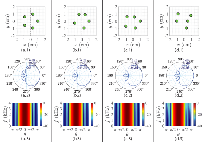

  

  Array geometries and the corresponding beampatterns of a first-order differential beamformer: a array geometry, b beampatterns at f=500 Hz, and c broadband beampattern versus frequency

• Array-II: an obtuse isosceles triangle array, the coordinates of the three microphones are (0,1.5),(−0.87,−0.5), and (0.87,−0.5), respectively, see Fig. 2(b.1).

• Array-III: an acute isosceles triangle array, the coordinates of the three microphones are (0,0.6), (−0.87,−0.5), and (0.87,−0.5), respectively, see Fig. 2(c.1).

• Array-IV: a scalene triangle array with top microphone being off the central axis, the coordinates of the three microphones are (0,1.04),(−0.87,−0.5), and (0.87,−0.5), respectively, see Fig. 2(d.1).

Figure 2 plots the four different geometries and the corresponding beampatterns, and broadband beampatterns versus frequency designed with the presented algorithm, where the desired look direction is 0^∘. As seen, the presented method successfully formed the first-order supercardioid for all the four geometries and the designed beampatterns are almost frequency invariant. Figure 3 plots the DIs and the WNGs of the designed differential beamformers with the aforementioned four array geometries. It is clearly seen that the DI does not change much with frequency for all the four geometries, indicating that the designed beampatterns are frequency invariant.

Fig. 3

DI and WNG of the first-order differential beamformer designed with the algorithm in (25) with four different array geometries: a DI and b WNG

Figure 4 plots the DIs and the WNGs for different look directions, θ_s, at f=1000 Hz. It is clearly seen that the DIs stay constant (approximately 5 dB) but the WNGs fluctuate with θ_s (except Array-I). The results confirm our previous conclusion that continuously steerable DMAs can be designed by using three microphones if they are not arranged in a linear manner. It is also observed from Fig. 4 that the WNGs for the four geometries are slightly different from each other. This result is interesting from a practical perspective. With the same number of microphones, we can form the same beampattern with the same DI while optimizing the geometry to improve the WNG.

Fig. 4

DI and WNG of the first-order differential beamformer with four different array geometries for different look directions. a DI and b WNG

6.2 Second-order DMAs

We then study the performance of the presented method for the design of second-order DMAs, where the desired target beampattern is the second-order supercardioid, and its coefficients are chosen according to Table 1. In the simulations, we use five microphones and consider the following four different array geometries (coordinate values measured in centimeters).

• Array-I : a regular pentagon array (also can be considered as a uniform circular microphone array), the coordinates of the five microphones are (1.0,0),(0.31,0.95),(−0.81,0.59),(−0.81,−0.59), and (0.31,−0.95), respectively, see Fig. 5(a.1).

  Fig. 5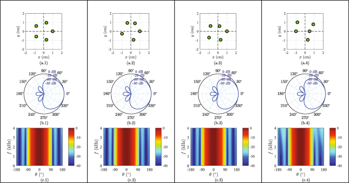

  

  Array geometries and the corresponding beampatterns of a second-order differential beamformer: a array geometry, b beampatterns at f=500 Hz, and c broadband beampattern versus frequency

• Array-II: a pentagon array where the radii of the microphones are the same but angles are nonuniform, the coordinates of the five microphones are (1.0,0),(0.47,0.88),(−0.38,0.93),(−0.96,−0.28), and (0.31,−0.95), respectively, see Fig. 5(b.1).

• Array-III: a pentagon array where the angles of microphones are uniform, but the radius are nonuniform, the coordinates of the five microphones are (1.0,0),(0.19,0.57),(−0.81,0.59),(−0.97,−0.71), and (0.31,−0.95), respectively, see Fig. 5(c.1).

• Array-IV: the coordinates of the microphones is randomly distributed, the coordinates of the five microphones are (0.5,0),(0.92,0.77),(1.0,0),(−0.84,1.0), and (0.31,−0.95), respectively, see Fig. 5(d.1).

Figure 5 plots the array geometries, the corresponding beampatterns, and broadband beampatterns versus frequency. It is clearly seen that the presented method successfully formed the second-order supercardioid for all the four geometries and the designed beampatterns are almost frequency invariant. Figure 6 plots the DIs and the WNGs as a function of frequency, where the DIs, again, stay constant but the WNGs increase with frequency. It is also seen that both the DIs and WNGs for the four geometries are different. This can be easily explained, and the DI is defined as the ratio between the magnitude-squared beampattern in the look direction and the averaged magnitude-squared beampattern over the entire space. But the beampattern is defined only in the sensor plane. As a result, the DIs are different even though beampatterns are the same. In our study, we focus on the 2-dimensional space with the assumption that the sound sources and the sensors are in the same plane. The designed beamformer will achieve good performance if the steering angles are within or near the sensor plane, but it becomes less and less effective as the beamformer is steered away from this plane. This problem has been fully studied with circular differential beamformers [54], and the conclusion also applies to other kinds of planar arrays.

Fig. 6

DI and WNG of the second-order differential beamformer designed with four different array geometries: a DI and b WNG

Figure 7 plots the DIs and WNGs as a function of θ_s at f=1000 Hz. It is seen that, for some geometries, the DI and WNG change with θ_s, which indicates that geometries play an important role on the steering capability of the beamformer. However, it should be noted that the beamformer is continuously steerable regardless of geometry.

Fig. 7

DI and WNG of the second-order differential beamformer designed with four different array geometries for different look directions: a DI and b WNG

6.3 Third-order DMAs

We then study the performance of the presented method for the design of a third-order supercardioid with M=7 and consider the following four different array geometries (coordinate values measured in centimeters).

• Array-I : a regular heptagon microphone array (also can be considered as a uniform circular microphone array), the coordinates of the seven microphones are (1.5,0),(0.94,1.17),(−0.34,1.46),(−1.35,0.66),(−1.35,−0.66),(−0.34,−1.46), and (0.94,−1.17), respectively, see Fig. 8(a.1).

  Fig. 8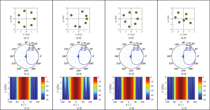

  

  Array geometries and the corresponding beampatterns of a third-order differential beamformer: a array geometry, b beampatterns at f=500 Hz, and c broadband beampattern versus frequency

• Array-II: a heptagon microphone array where the angle positions of microphones are nonuniform, but the radii are the same, and the coordinates of the seven microphones are (1.5,0),(1.40,0.54),(0.68,1.34),(−1.35,0.66),(−0.61,−1.37),(0.18,−1.49), and (1.29,−0.77), respectively, see Fig. 8(b.1).

• Array-III: a heptagon microphone array where the radii of the microphones are nonuniform, but the angle positions are the same, and the coordinates of the seven microphones are (1.2,0),(0.94,1.17),(−0.27,1.17),(−1.35,0.66),(−1.08,−0.53),(−0.34,−1.46), and (0.76,−0.93), respectively, see Fig. 8(c.1).

• Array-IV: the coordinates of the microphones are randomly distributed, and the coordinates of the seven microphones are (0.5,0),(0.5,0.87),(−0.96,1.15),(−1.48,0.26),(−0.77,−0.64),(0.05,−0.30), and (1.29,−0.77), respectively, see Fig. 8(d.1).

Figure 8 plots the four different geometries and the corresponding beampatterns and broadband beampatterns versus frequency. Figure 9 plots the DIs and the WNGs as a function of frequency, f. Similarly, with all the four array geometries, the presented method successfully formed the third-order supercardioid and the designed beampatterns are almost frequency invariant. The designed third-order DMA is continuously steerable, with a constant DI; but the DIs and WNGs are different for the four geometries.

Fig. 9

DI and WNG of the third-order differential beamformer designed with four different array geometries: a DI and b WNG

6.4 Robust DMAs

As seen, the DI and the WNG fluctuate with the steering direction. This can be improved by increasing the number of microphones and designing the beamformer with the minimum-norm solution. To demonstrate this, we show an example for the design of robust DMAs with M=25, where the coordinates of the microphones are random numbers generated with the uniform distribution by confining 1≤r_m≤2 cm and −π<ψ_m≤π. Figure 10 plots the DIs and the WNGs as a function of the steering direction, θ_s and f, of the designed second- and third-order supercardioid, respectively. Now, it is clearly seen both the DIs and the WNGs are almost constant. Clearly, the performance can be further improved if more microphones are used.

Fig. 10

DI and WNG of the robust differential beamformer for different look directions: a DI and b WNG

Note that there may exist some errors when implementing the beamformer with limited precision in practice. This effect can be modeled by WNG, which evaluates the performance of a beamformer with respect to the presence of array imperfection as well as other uncertainties. So, one can deal with such errors by improving the WNG.

6.5 Experiments in real environment

In this subsection, we present an example of using the proposed DMA beamformer in a real office room environment. The size of the office room is approximately 3×4×3 m, where the reverberation time, T₆₀, which is computed from a measured room impulse response, is approximately 600 ms. A loudspeaker is placed 1 m away from the array with an elevation angle of 30^∘, which plays back a prerecorded speech signal to simulate a sound source of interest. Note that this source position is arbitrarily selected. The acoustic scenario for the experiments also consists of air conditioning noise, environmental noise from outside of the windows, and some babble noise from another working area, which is over 6 m away. The overall signal-to-noise-ratio (SNR), which is evaluated from the reference microphone, is approximately 4.5 dB. We first built a concentric circular microphone array, which consists of 7 sensors, a photo of which is shown in Fig. 11. We then choose 4 microphones from the array to form an irregular geometry array, where the 4 used microphones are marked with a circle. We choose the center of the four microphones as the reference point, the coordinates (measured in centimeters) of the four microphones are (1.9,0),(0,3.29),(−1.9,0), and (0,3.29), respectively. The DMA is expected to be mounted in the head of a robot (however, due to logistic issues, in this experiment, the DMA is mounted on a tripod). The desired source is in a randomly selected direction (a loudspeaker about 1 m away and with elevation angle of 30^∘ to play back a speech signal of interest).

Fig. 11

A photo of the designed microphone arrays and the used irregularity microphone array with 4 microphones (marked with a circle)

The microphone outputs are first passed through a preamplifier and then fed to a 24-bit analog-to-digital converter with a sampling rate of 8 kHz. Then, the digitized signals are then processed with a TI floating-point processor. The beamformers are implemented in the STFT domain with a frame size of 32 ms (256 points) and an overlapping factor of 75% (a Kaiser window is applied to each frame). The beamforming filters are computed according to (25) with the target beampattern as the 1st-order cardioid. Figure 12 plots the time-domain observed signal and its spectrogram and the output of the developed DMA beamformer and its spectrogram. It is seen that the output of the DMA enhanced the desired signal and suppressed reverberation and noise, which indicates the effectiveness of the developed beamformer.

Fig. 12

Performance in a conference room: a signal observed at the 1st sensor and its spectrogram and b output of the 1st-order DMA beamformer and its spectrogram

6.6 Comparison

As discussed previously, with a fixed array geometry and number of microphones, we can improve the DMA performance by choosing an appropriate reference point, i.e., making the value of r_m as small as possible. We present two examples for the design of supercardioids using the conventional method in [51], i.e., (26), and the proposed method, i.e., (29), respectively, in Fig. 13, where we use a uniform linear microphone array consisting of four closely spaced microphones with the interelement spacing being 1 cm. As seen, the beampattern of the linear DMA designed by the proposed method matches better the target beampattern than the beampattern designed with the conventional method. It is clearly seen that the proposed method achieves better performance as compared to the conventional method [51].

Fig. 13

Beampatterns designed with the conventional method in [51] and the proposed method: a the target beampattern (second-order supercardioid), b conventional method, and c proposed method

The proposed method is also compared to the conventional null-constrained differential beamformer in [37], where we use Array-I as shown in Fig. 2(a,1), and the desired beampattern is the first-order supercardioid with θ_s=130^∘. The results are plotted in Fig. 14. For reference, the performance of the delay-and-sum (DS) beamformer is also plotted. As seen, while the DS beamformer has a large WNG, its directivity is very small. In comparison, the differential beamformers have much higher DIs, which are almost frequency-invariant. It is also seen that the proposed method achieves higher DIs than the conventional null-constrained differential beamformer.

Fig. 14

DI and WNG of the proposed differential beamformer, the conventional null-constrained differential beamformer in [37], and the DS beamformer: a DI and b WNG

7 Conclusions

Towards robotic applications, where microphone arrays face restrictions in size and geometry, we presented in this paper an approach to the design of differential beamformers with arbitrary planar array geometries. By approximating the beampattern with the Jacobi-Anger expansion, we developed an algorithm that can form beampatterns close to a pre-specified target frequency-invariant beampattern. This method is rather general and it can be used to design differential beamformers with linear, circular, concentric circular DMAs, and arrays where sensors are placed in any specified positions. Based on the proposed method, some basic requirements for the design of first-, second-, and third-order LDMAs, LSDMAs, and CSDMAs were discussed. This study also summarized the fundamental requirements, i.e., the number of microphones and array geometries, for the design of different kinds and orders of DMAs.

8 \thelikesection Appendix A

9 \thelikesection Derivation of the column rank of Ψ^H(ω)

In case 2N, microphones are uniformly distributed on a circular array, and the vector ψ_n(ω) defined in (19) can be written as

$$\begin{array}{*{20}l} \boldsymbol{\psi}_{n} (\omega) &= J_{n} \left(\omega r/c \right) \boldsymbol{\psi}'_{n} (\omega), \end{array} $$

(41)

with

$$\begin{array}{*{20}l} \boldsymbol{\psi}'_{n} &= \left[ e^{-\jmath n \psi_{1}} ~~ e^{-\jmath n \psi_{2} } \cdots ~~ e^{-\jmath n \psi_{M}} \right]^{T}. \end{array} $$

(42)

Since M=2N, it is clear that the mth element of vectors ψ−N′ and ψN′ are

$$\begin{array}{*{20}l} \boldsymbol{\psi}'_{-N,m} &= e^{\jmath N \psi_{m} } = e^{\jmath \frac{M}{2}\frac{2 \pi}{M} (m-1) } = \cos\left[ (m-1) \pi \right], \\ \boldsymbol{\psi}'_{N,m} &= e^{-\jmath N \psi_{m} } = \cos\left[ (m-1) \pi \right]. \end{array} $$

(43)

From (43), it is clearly seen

$$\begin{array}{*{20}l} \boldsymbol{\psi}'_{-N} &= \boldsymbol{\psi}'_{N}. \end{array} $$

(44)

So, we have

$$\begin{array}{*{20}l} \boldsymbol{\Psi}(\omega) \boldsymbol{\Psi}^{H}(\omega) &= M \mathbf{J}(\omega) \mathbf{P}, \end{array} $$

(45)

where

$$\begin{array}{*{20}l} \mathbf{J}(\omega) &= \text{diag} \left[ J_{-N}^{2} \left(\omega r/c \right), \ldots, J_{0}^{2} \left(\omega r/c \right), \ldots, J_{N}^{2} \left(\omega r/c \right) \right] \end{array} $$

(46)

is a (2N+1)×(2N+1) diagonal matrix, and

$$\begin{array}{*{20}l} \mathbf{P} &= \left[ \begin{array}{ccccc} 1 & 0 & \cdots & 0 & 1 \\ 0 & 1 & \cdots & 0 & 0 \\ \vdots & \vdots & \ddots & \vdots & \vdots \\ 0 & 0 & \cdots & 1 & 0 \\ 1 & 0 & \cdots & 0 & 1 \\ \end{array} \right] = \left[ \begin{array}{ccccc} \mathbf{I}_{2N} & \mathbf{i}_{1} \\ \mathbf{i}^{T}_{1} & 1 \end{array} \right], \end{array} $$

(47)

with I_2N being the 2N×2N identity matrix and i₁ being the first column of the I_2N. It is clearly seen that rank(P)=2N. Then,

$$\begin{array}{*{20}l} {\mathcal{R}} \left[ \boldsymbol{\Psi}(\omega) \boldsymbol{\Psi}^{H}(\omega) \right] &= 2N, \end{array} $$

(48)

where ${\mathcal {R}}$ denotes the column rank of a matrix. As a consequence, we have

$$\begin{array}{*{20}l} {\mathcal{R}} \left[ \boldsymbol{\Psi}^{H}(\omega) \right] &\geq 2N. \end{array} $$

(49)

According to (44), it is also clear that

$$\begin{array}{*{20}l} {\mathcal{R}} \left[ \boldsymbol{\Psi}^{H}(\omega) \right] & \leq 2N. \end{array} $$

(50)

According to (49) and (50), we get (31), i.e., the column rank of Ψ^H(ω) is 2N.

References

H. W. Löllmann, A. Moore, P. A. Naylor, B. Rafaely, R. Horaud, A. Mazel, W. Kellermann, in HSCMA. Microphone array signal processing for robot audition (IEEESan Francisco, 2017), pp. 51–55.
K. Sekiguchi, Y. Bando, K. Nakamura, K. Nakadai, K. Itoyama, K. Yoshii, in IEEE/RSJ IROS. Online simultaneous localization and mapping of multiple sound sources and asynchronous microphone arrays (IEEEDaejeon, 2016), pp. 1973–1979.
C. Evers, Y. Dorfan, S. Gannot, P. A. Naylor, in Proc. IEEE ICASSP. Source tracking using moving microphone arrays for robot audition (IEEENew Orleans, 2017), pp. 6145–6149.
H. Barfuss, M. Bachmann, M. Buerger, M. Schneider, W. Kellermann, in Proc. IEEE WASPAA. Design of robust two-dimensional polynomial beamformers as a convex optimization problem with application to robot audition (IEEENew Paltz, 2017), pp. 106–110.
H. Barfuss, M. Buerger, J. Podschus, W. Kellermann, in HSCMA. HRTF-based two-dimensional robust least-squares frequency-invariant beamformer design for robot audition (IEEESan Francisco, 2017), pp. 56–60.
J. Benesty, I. Cohen, J. Chen, Fundamentals of signal enhancement and array signal processing (John Wiley & Sons, 2018).
G. Huang, J. Chen, J. Benesty, On the design of differential beamformers with arbitrary planar microphone array. J. Acoust. Soc. Am.144(1), 66–70 (2018).
J. Benesty, J. Chen, Y. Huang, Microphone array signal processing (Springer-Verlag, Berlin, Germany, 2008).
S. Gannot, D. Burshtein, E. Weinstein, Analysis of the power spectral deviation of the general transfer function GSC. IEEE Trans. Signal Process.52:, 1115–1120 (2004).
S. Yan, Y. Ma, C. Hou, Optimal array pattern synthesis for broadband arrays. J. Acoust. Soc. Am.122(5), 2686–2696 (2007).
B. Rafaely, D. Khaykin, Optimal model-based beamforming and independent steering for spherical loudspeaker arrays. IEEE Trans. Audio, Speech, Lang. Process.19(7), 2234–2238 (2011).
S. Yan, Optimal design of modal beamformers for circular arrays. J. Acoust. Soc. Am.138(4), 2140–2151 (2015).
B. Rafaely, Fundamentals of spherical array processing (Springer-Verlag, Berlin, Germany, 2015).
E. D. Sena, H. Hacihabiboglu, Z. Cvetkovic, On the design and implementation of higher-order differential microphones. IEEE Trans. Audio, Speech, Lang. Process.20:, 162–174 (2012).
M. Buck, Aspects of first-order differential microphone arrays in the presence of sensor imperfections. European Trans. Telecomm.13(2), 115–122 (2002).
G. Huang, J. Benesty, I. Cohen, J. Chen, Differential beamforming on graphs. IEEE/ACM Trans. Audio, Speech, Lang. Process.28(1), 901–913 (2020).
A. Bernardini, F. Antonacci, A. Sarti, Wave digital implementation of robust first-order differential microphone arrays. IEEE Signal Process. Lett.25(2), 253–257 (2017).
F. Borra, A. Bernardini, F. Antonacci, A. Sarti, Uniform linear arrays of first-order steerable differential microphones. IEEE/ACM Trans. Audio, Speech, Lang. Process.27(12), 1906–1918 (2019).
F. Borra, A. Bernardini, F. Antonacci, A. Sarti, Efficient implementations of first-order steerable differential microphone arrays with arbitrary planar geometry. IEEE/ACM Trans. Audio, Speech, Lang. Process. (2020).
G. Huang, J. Chen, J. Benesty, in Proc. IEEE ICASSP. On the design of robust steerable frequency-invariant beampatterns with concentric circular microphone arrays (IEEECalgary, 2018), pp. 506–510.
E. Tiana-Roig, F. Jacobsen, E. F. Grande, Beamforming with a circular microphone array for localization of environmental noise sources. J. Acoust. Soc. Am.128(6), 3535–3542 (2010).
E. Tiana-Roig, F. Jacobsen, E. Fernandez-Grande, Beamforming with a circular array of microphones mounted on a rigid sphere (L). J. Acoust. Soc. Am.130(3), 1095–1098 (2011).
A. M. Torres, M. Cobos, B. Pueo, J. J. Lopez, Robust acoustic source localization based on modal beamforming and time–frequency processing using circular microphone arrays. J. Acoust. Soc. Am.132(3), 1511–1520 (2012).
G. W. Elko, Microphone array systems for hands-free telecommunication. Speech Commun.20(3), 229–240 (1996).
G. W. Elko, J. Meyer, in Springer Handbook of Speech Processing, ed. by J. Benesty, M. M. Sondhi, and Y. Huang. Microphone arrays (Springer-VerlagBerlin, Germany, 2008), pp. 1021–1041. Chap. 48.
J. Benesty, J. Chen, Study and design of differential microphone arrays (Springer-Verlag, Berlin, Germany, 2012).
G. Huang, J. Chen, J. Benesty, Design of planar differential microphone arrays with fractional orders. IEEE/ACM Trans. Audio, Speech, Lang. Process.28:, 116–130 (2019).
J. Benesty, I. Cohen, J. Chen, Array processing-Kronecker product beamforming (Springer-Verlag, Berlin, Germany, 2019).
I. Cohen, J. Benesty, J. Chen, Differential Kronecker product beamforming. IEEE/ACM Trans. Audio, Speech, Lang. Process.27(5), 892–902 (2019).
Y. Buchris, I. Cohen, J. Benesty, A. Amar, Joint sparse concentric array design for frequency and rotationally invariant beampattern. IEEE/ACM Trans. Audio, Speech, Lang. Process.28:, 1143–1158 (2020).
Y. Buchris, I. Cohen, J. Benesty, Frequency-domain design of asymmetric circular differential microphone arrays. IEEE/ACM Trans. Audio, Speech, Lang. Process.26(4), 760–773 (2018).
G. Huang, J. Benesty, I. Cohen, J. Chen, A simple theory and new method of differential beamforming with uniform linear microphone arrays. IEEE/ACM Trans. Audio, Speech, Lang. Process.28(1), 1079–1093 (2020).
G. W. Elko, A. -T. N. Pong, in Proc. IEEE ICASSP, 1. A steerable and variable first-order differential microphone array (IEEEMunich, 1997), pp. 223–226.
R. M. Derkx, K. Janse, Theoretical analysis of a first-order azimuth-steerable superdirective microphone array. IEEE Trans. Audio, Speech, Lang. Process.17(1), 150–162 (2009).
X. Wu, H. Chen, J. Zhou, T. Guo, Study of the mainlobe misorientation of the first-order steerable differential array in the presence of microphone gain and phase errors. IEEE Signal Process. Lett.21(6), 667–671 (2014).
X. Wu, H. Chen, Directivity factors of the first-order steerable differential array with microphone mismatches: deterministic and worst-case analysis. IEEE/ACM Trans. Audio, Speech, Lang. Process.24(2), 300–315 (2016).
J. Benesty, J. Chen, I. Cohen, Design of circular differential microphone arrays (Springer-Verlag, Berlin, Germany, 2015).
J. Byun, Y. C. Park, S. W. Park, Continuously steerable second-order differential microphone arrays. J. Acoust. Soc. Am.143(3), 225–230 (2018).
A. Bernardini, M. D. Aria, R. Sannino, A. Sarti, Efficient continuous beam steering for planar arrays of differential microphones. IEEE Signal Process. Lett.24(6), 794–798 (2017).
G. Huang, J. Benesty, J. Chen, On the design of frequency-invariant beampatterns with uniform circular microphone arrays. IEEE/ACM Trans. Audio, Speech, Lang. Process.25(5), 1140–1153 (2017).
G. Huang, J. Chen, J. Benesty, Insights into frequency-invariant beamforming with concentric circular microphone arrays. IEEE/ACM Trans. Audio, Speech, Lang. Process.26(12), 2305–2318 (2018).
L. C. Parra, in Proc. IEEE WASPAA. Least squares frequency-invariant beamforming (IEEENew Paltz, 2005), pp. 102–105.
L. C. Parra, Steerable frequency-invariant beamforming for arbitrary arrays. J. Acoust. Soc. Am.119(6), 3839–3847 (2006).
C. C. Lai, S. Nordholm, Y. H. Leung, Design of steerable spherical broadband beamformers with flexible sensor configurations. IEEE Trans. Audio, Speech, Lang. Process.21(2), 427–438 (2013).
Y. Wang, Y. Yang, Z. He, Y. Han, Y. Ma, A general superdirectivity model for arbitrary sensor arrays. EURASIP J. Adva. Signal Process.2015(1), 68 (2015).
A. Medda, A. Patel, in 2017 51st Asilomar Conference on Signals, Systems, and Computers,. Frequency invariant beamforming for arbitrary planar arrays (Pacific Grove, 2017), pp. 1133–1136.
H. V. Trees, Optimum array processing: part IV of detection, estimation, and modulation theory (John Wiley Sons, Inc, New York, 2002).
M. Brandstein, D. Ward, microphone arrays: signal processing techniques and applications (Springer, 2001).
G. W. Elko, in Audio signal processing for next-generation multimedia communication systems. Differential microphone arrays (Springer, 2004), pp. 11–65.
M. Abramowitz, I. A. Stegun, Handbook of mathematical functions: with formulas, graphs, and mathematical tables, vol. 55 (Dover Publications, New York, 1965).
L. Zhao, J. Benesty, J. Chen, Design of robust differential microphone arrays with the Jacobi–Anger expansion. Appl. Acous.110:, 194–206 (2016).
G. Huang, J. Benesty, J. Chen, Design of robust concentric circular differential microphone arrays. J. Acoust. Soc. Am.141(5), 3236–3249 (2017).
H. Zhang, J. Chen, J. Benesty, Study of nonuniform linear differential microphone arrays with the minimum-norm filter. Appl. Acous.98:, 62–69 (2015).
G. Huang, X. Zhao, J. Chen, J. Benesty, in Proc. IEEE ICASSP. Properties and limits of the minimum-norm differential beamformers with circular microphone arrays (IEEE, 2019), pp. 426–430.
Acknowledgements
This work was supported in part by the NSFC Distinguished Young Scientists Fund (grant no. 61425005), Israel Science Foundation (grant no. 576/16), and the ISF-NSFC joint research program (grant No. 2514/17 and 61761146001).
Author information
Authors and Affiliations
Contributions
The authors read and approved the final manuscript.
Corresponding author
Ethics declarations
Competing interests
The authors declare that they have no competing interests.
Additional information
Publisher’s Note
Springer Nature remains neutral with regard to jurisdictional claims in published maps and institutional affiliations.
Rights and permissions
Open Access This article is licensed under a Creative Commons Attribution 4.0 International License, which permits use, sharing, adaptation, distribution and reproduction in any medium or format, as long as you give appropriate credit to the original author(s) and the source, provide a link to the Creative Commons licence, and indicate if changes were made. The images or other third party material in this article are included in the article’s Creative Commons licence, unless indicated otherwise in a credit line to the material. If material is not included in the article’s Creative Commons licence and your intended use is not permitted by statutory regulation or exceeds the permitted use, you will need to obtain permission directly from the copyright holder. To view a copy of this licence, visit http://creativecommons.org/licenses/by/4.0/.
About this article
Cite this article
Huang, G., Chen, J., Benesty, J. et al. Steerable differential beamformers with planar microphone arrays. J AUDIO SPEECH MUSIC PROC. 2020, 15 (2020). https://doi.org/10.1186/s13636-020-00185-1
Received:
Accepted:
Published:
DOI: https://doi.org/10.1186/s13636-020-00185-1