Dynamic out-of-vocabulary word registration to language model for speech recognition

Abstract

We propose a method of dynamically registering out-of-vocabulary (OOV) words by assigning the pronunciations of these words to pre-inserted OOV tokens, editing the pronunciations of the tokens. To do this, we add OOV tokens to an additional, partial copy of our corpus, either randomly or to part-of-speech (POS) tags in the selected utterances, when training the language model (LM) for speech recognition. This results in an LM containing OOV tokens, to which we can assign pronunciations. We also investigate the impact of acoustic complexity and the “natural” occurrence frequency of OOV words on the recognition of registered OOV words. The proposed OOV word registration method is evaluated using two modern automatic speech recognition (ASR) systems, Julius and Kaldi, using DNN-HMM acoustic models and N-gram language models (plus an additional evaluation using RNN re-scoring with Kaldi). Our experimental results show that when using the proposed OOV registration method, modern ASR systems can recognize OOV words without re-training the language model, that the acoustic complexity of OOV words affects OOV recognition, and that differences between the “natural” and the assigned occurrence frequencies of OOV words have little impact on the final recognition results.

1 Introduction

The language models (LMs) of automatic speech recognition (ASR) systems are often trained statistically using corpora with fixed vocabularies. Thus, when applying ASRs (e.g., in dialog systems), we always encounter out-of-vocabulary (OOV) words such as the names of new movie stars or new Internet slang, such as “jsyk” (just so you know). This can be problematic since such OOV words are often closely related to the main topic being discussed. Accurate recognition of these OOV words would undoubtedly result in a huge improvement in the accuracy of ASR-based sentence understanding systems.

Subword acoustic models are often used to recognize OOV words. For example, phone models have been used with a phone bigram to recognize arbitrary phone sequences [1]. Morphemes have also been used as subwords [2, 3]. This kind of “speech typewriter” cannot achieve comparative OOV word recognition performance as can be achieved for in-vocabulary words, however.

Another approach to tackling the OOV problem is OOV detection. In the 2000’s, various OOV detection methods were proposed, most of them based on confidence measures. Various acoustic and linguistic features were fed into, for example, a Fisher Linear Discriminant Analysis (FLDA)-based classifier [4] to classify speech regions into OOVs and IVs (in-vocabulary words). Decoding graph information and semantic information were also used to classify OOVs and IVs within a boosting classification algorithm [5]. Word/subword hybrid systems were also used for OOV word detection [6]. In [7], the OOV word detection task was treated as a sequence labeling problem. A MaxEnt classifier used additional features, based on the local lexical context, as well as global features from a language model using the entire utterance. In another study, OOVs were detected by searching a confusion network [8]. After detection, recovery of the OOV word is generally performed [9, 10]. These approaches can be used to recognize OOV words, but recovery often fails due to a lack of lexical information. Thus, when we want to recognize particular, known words which are unknown to both the language model and the dictionary used in the speech recognizer, it is better to register the words to the model and the dictionary.

If the system can reference OOV words, it is better to use an LM which includes these words. One possible way to create an LM which includes OOV words is to use training data which includes these words. Such training data is often created by gathering text from the web or by replacing words similar to the OOV words in the data with the targeted OOV words. However, as LMs become more and more complex, training them takes more and more time. Therefore, the ability to dynamically add new words to LMs without re-training is considered to be a necessary feature of modern ASR systems. The most common approach used to dynamically update LMs is to assign probabilities to OOV words. This is achieved by modifying the LM’s probability distribution. These methods attempt to assign the parameters of OOV words to the existing LM along with their meanings and part-of-speech (POS) tags. For example, in [11, 12], researchers proposed using similar, in-vocabulary (IV) words to estimate the N-gram probabilities of OOV words. Recently, word embedding has been adopted to measure the similarity between IV and OOV words [13]. Some researchers have tackled this problem using word class N-grams [14]. In [15], a probability was assigned to OOV words based on a word class whose probability had already been determined. These approaches have achieved a modest level of performance, but the system must have some kind of semantic knowledge to measure the similarities and determine which class the OOV words should be assigned to. When using a class N-gram, words in each class share a class probability, while the probability of each word is approximated by combining the class probability and the target word’s probability within the class; thus, word probability estimation is degraded, resulting in the performance of the speech recognition system also being degraded. Moreover, our proposed method can be used in speech recognition systems which do not support class N-grams.

Alternatively, we propose a simple but powerful corpus modification method in which we artificially add OOV tokens during the training of the language model, creating an LM with OOV tokens chosen a priori. The system then registers OOV words to the positions of the OOV tokens in the LM, resulting in an LM which includes the OOV words. For example, to train an LM, we create a training corpus by inserting or replacing some words with OOV tokens. After training the LM using this corpus, we obtain an LM containing OOV tokens. To apply this LM to speech recognition, we replace OOV tokens with words which are not contained in the pronunciation dictionary (i.e., OOV words). When using our method, degradation of the estimation of in-vocabulary word probabilities is suppressed to the minimum, because the probability of each OOV and IV word is estimated. As part of this study, we investigated how OOV tokens could be added to the training data. Since ASR systems create recognition hypotheses based on the output probabilities of both their acoustic models (AMs) and their LMs, the impact of the acoustic complexity of OOV words on OOV word recognition is unclear, although one might assume that OOV words with “unique” pronunciations are easier to recognize. In this paper, we define the acoustic complexity of a word using the number of moras in the word. That is, the greater the number of moras, the more complex the word is. Finally, since OOV words should have a “natural” occurrence frequency (i.e., the frequency of their occurrence in a virtual, universal corpus), the impact of the difference between an OOV word’s “natural” probability and its assigned probability for OOV word recognition also needs to be investigated. The present study aims to supply global answers to all of these questions by experimentally investigating recognition of simulated OOV words using two popular modern ASR systems.

2 Dynamic OOV registration

2.1 Method

In our proposed method, we first train a language model using a corpus which includes OOV tokens. These OOV tokens are inserted into the corpus artificially, and thus, each OOV token appears as both a context word and a target word in the LM. Then, when using the LM in the recognition phase, the target OOV word pronunciations which the user wants the recognizer to recognize are assigned to the OOV tokens. This is realized by editing the pronunciations of the OOV tokens. Immediately after training the LM, the OOV tokens do not have any associate pronunciations. To assign a particular OOV token to a particular target to be recognized, we edit the pronunciation dictionary to link the OOV token to the pronunciation of the target word. The merit of our method is its ability to control the frequency of OOV occurrences. The more OOV tokens we insert, the larger the probabilities that can be assigned to the OOV words. In addition, OOV words can be added to the LM without the need for re-training.

The procedure used by the proposed method is as follows:

• 1 Make a partial copy of the corpusm, to be used for OOV token insertion. This procedure is optional, because OOV tokens can also be inserted into original corpus, but in our experiment, we first made a copy of some of the sentences and insert the OOV tokens into the copied sentences, as describe in the next step.

• 2 Add OOV tokens (e.g., “OOV1,” “OOV2,” $\dots$, “OOV _N”) to the utterances in the copied corpus, in order to generate “additional utterances.”

• 3 Use the corpus and the additional utterances to train the language model. As a result of this procedure, we obtain an LM which includes OOV tokens.

• 4 Edit the pronunciations of the tokens for the particular OOV words we want to register. Generally, a pronunciation dictionary is created for all of the in-vocabulary words of the LM, but pronunciations are not assigned to any of the OOV tokens. In our method, we edit the dictionary to assign the pronunciations we would like to recognize to the associated tokens.

• 5 Perform speech recognition.

An illustration of the editing of the pronunciation dictionary is shown in Fig. 1. One of the key points to be determined when using our method is where the OOV tokens should be inserted. Thus, we compared the effectiveness of using the following two methods in step 2:

• Random insertion—one token is added to each “additional utterance” at a random location

  Fig. 1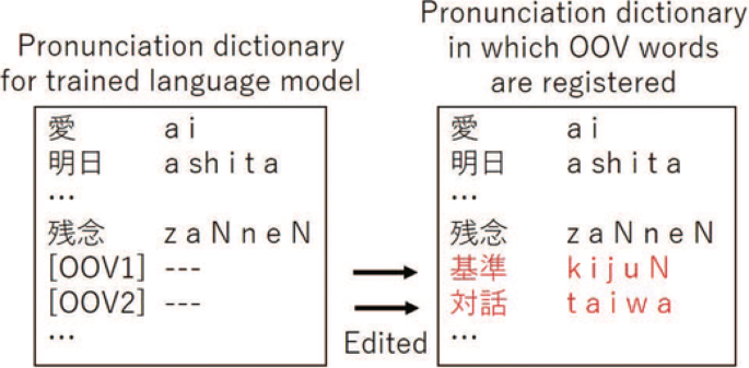

  

  An example of OOV word registration

• POS tag-based replacement—one word is replaced in each “additional utterance” whose POS tag is the same as the token’s POS tag

The proposed method can dynamically register new OOV words by editing the pronunciations of the OOV tokens. Different types of OOV tokens for OOV words with different properties (properties which are assumed to be known, e.g., acoustic complexity and POS tag) can also be prepared. For example, under the random insertion condition only, the pronunciation of the OOV words was assumed to be known, while under the POS tag-based replacement condition, we assumed that we knew each OOV word’s POS and pronunciation.

2.2 Impact of word properties

The impact of using each of these two types of word properties (acoustic complexity and POS tag) on the proposed OOV registration method is also investigated in the experiment phase of this study. To investigate the impact of the acoustic complexity of the OOV words, we defined four levels of acoustic complexity, which were measured according to the number of moras the OOV words contained, which could range from 2 to 5 moras. To investigate the impact of the difference between the “natural” and assigned probabilities of the OOV words, we evaluated four different insertion scales (i.e., the number of utterances generated for each OOV token), which were either 500, 1000, 2000, or 5000 utterances. During the experimental phase, we inserted four different OOV tokens at each level of acoustic complexity to generate additional utterances for each insertion scale condition and each registration condition (i.e., random and POS tag based), to be used to register the words in Table 1. All of these additional utterances were then used to train the LM, along with the basic corpus, which means that we added (500+1000+2000+5000)×2×4=68,000 additional utterance to our corpus. As the number of utterances in the original corpus was about 440,000, the additional utterances were equal to one sixth of the original corpus.

Table 1 Selected out-of-vocabulary (OOV) words and their frequency of occurrence

We also set two baseline conditions in our experiment: ONE and ALL. Under the ONE condition, the LM is trained using the basic corpus, which includes only pronunciation information and the smoothing probability of the OOV words given by the LM toolkit. Under this condition, only very rare words lacking sufficient statistical confidence are removed and replaced with OOV tokens; thus, only a small number of OOV tokens remain in the corpus. In our experiment, words with an occurrence frequency of 1 were removed. As a result, the probabilities of the N-gram model corresponding to the OOV words becomes small, but Kneser-Ney smoothing gives them some level of probability. Under the ALL condition, which is considered to be the ideal condition, the LM is trained using the original corpus which includes all of the selected OOV words.

3 Experimental setup

3.1 Data

The Corpus of Spontaneous Japanese (CSJ) [16] was selected to be the original corpus used in our experiment. It contains speech signals from speeches delivered in Japanese at domestic conferences. The corpus includes transcriptions of about 7 million words, along with various annotations such as POS and phonetic labels. In our experiment, we used the entire training set of the CSJ as our original corpus, which has a total length of 240 h and consists of 986 speeches. It contains about 440,000 utterances, with a vocabulary of around 70,000 words. For recognition, CSJ evaluation Set 1 (one of three available CSJ evaluation sets) was used, which contains 10 different lectures with a total of 1272 utterances (about 26,000 words). The total length of the test set was approximately 2 h.

We randomly selected 16 words as our OOV words, based on their acoustic complexity and occurrence frequency in the evaluation set, all of which were nouns¹. The selected words and their occurrence frequency in the corpora are shown in Table 1². Four words were selected for each level of acoustic complexity, and the average recognition/detection accuracy of these four words was used to evaluate the performance of the proposed OOV registration method with OOV words of that level of acoustic complexity. Note that in each recognition trial, we attempted to register and recognize each of the four OOV words at each level of acoustic complexity (all 16 words), at that particular insertion scale. Because we found it challenging to find enough words with 2 moras, we decided to use two words with multiple pronunciations, some of which contain a different number of moras. Both the word (“six”) and the word (“sound”) have multiple pronunciations. can be pronounced “roku,” “mui,” “muq,” “ro,” “riku,” or “muyu.” Except for “ro,” all of these pronunciations have 2 moras. Likewise, can be pronounced “oto,” “iN,” “oN,” or “ne.” Except for “ne,” all of these pronunciations have 2 moras. The utterances in the evaluation set, including OOV words, can be divided according to their level of acoustic complexity as follows: 58 are 2 mora words, 69 are 3 mora words, 49 are 4 mora words, and 41 are 5 mora words³.

3.2 Automatic speech recognition systems

We used the Julius [17] and Kaldi [18] ASR systems in our experiments. The Julius toolkit provides a pre-trained, deep neural network (DNN) hidden Markov model (HMM) for acoustic modeling (AM), which uses a corpus of Japanese newspaper article sentences (JNAS) and part of the CSJ speech corpus (simulated speech) as training data. For its language model, we used a forward bi-gram plus backward tri-gram LM, trained using SRILM [19] with entries (uni-gram/bi-gram/tri-gram) that appear more than one time, as well as modified Kneser-Ney smoothing for back-off. Since Julius is a classical decoder which directly uses acoustic models and N-gram language models, we can register new words only by changing the pronunciations of the OOV tokens.

The Kaldi toolkit provides several example training/test pipelines for different corpora, including the CSJ corpus which was used in our experiment. In particular, linear discriminant analysis (LDA) and maximum likelihood linear transform (MLLT) were used to process the original Mel-frequency cepstrum coefficient (MFCC) features. These processed MFCC features were then used as the input (basic features) for DNN-HMM training. A forward tri-gram LM with similar training conditions as those used to train the LM for the Julius ASR was also used as one of the Kaldi LMs. In this case, we had to compose Finite State Transducers (FSTs) a priori. Thus, in the training phase, we made a lexicon file (called “L.fst” in the Kaldi toolkit) and a grammar file (“G.fst”) first, using the training data, which included the OOV tokens with their tentative pronunciations. Next, we constructed anew L.fst file using the lexicon in which particular OOV word pronunciations were registered to the OOV tokens. We then composed it with the other FSTs to create the final FST (“HCLG. fst”). When using a WFST-based ASR system such as Kaldi, it is not as easy to register OOV words to the lexicon as it is with classical decoders. On the other hand, we do not need to retrain the language model using a huge text corpus that includes particular OOV words. A recurrent neural network (RNN)-based LM was also introduced as an alternative LM for Kaldi, specifically, the N-gram plus RNN re-scoring LM proposed in [20]. The RNN LM was used to calculate the scores of the N-best hypotheses provided by the N-gram LM. We trained the RNN language model using a text corpus with OOV tokens. In the testing phase, we viewed the OOV tokens as particular OOV words; thus, we could re-score the hypothesis including the particular OOV words using the RNN language model. The output scores of the RNN LM were then linearly interpolated with the scores provided by the original N-gram LM using the follow equation:

$$ P(h_{i})=\lambda P_{N} (h_{i})+(1-\lambda) P_{R} (h_{i}), $$

(1)

where P(h_i) is the final LM score of hypothesis i, P_N(h_i) is the probability calculated by the N-gram LM, P_R(h_i) is the probability calculated by the RNN LM, and λ is the interpolation weight which was set to 0.5 in our experiment⁴. Other details of the RNN LM used in this study are shown in Table 2

Table 2 Experimental conditions for the RNN language model

As mentioned above, we added a relatively large number of additional utterances containing our OOV words to the basic corpus, so the speech recognition word error rates (WERs) of the Julius and Kaldi N-gram LMs used in our experiment were both a bit higher (i.e., worse) than the reported best WERs for these ASRs, which are 29.20% and 17.07%, respectively. RNN LM re-scoring improved Kaldi’s WER to 14.23%.

3.3 Evaluation method

Recognition accuracy in our experiments was measured using utterance level false rejection rates (FRR) and false alarm rates (FAR) when the ASRs interpreted OOV utterances during the experiment. If OOV words were successfully recognized, the utterance containing this OOV word was counted as one “hit” (true positive, TP); if the ASR system did not recognize the OOV word, it was counted as one “miss” (false negative, FN); if the ASR system did not recognized any OOV words in an utterance without an OOV word, it was counted as one “correct dismissal” (true negative, TN); and finally, if the ASR system recognized any OOV words in an utterance without an OOV word, it was counted as one “false alarm” (false positive, FP). The false rejection rate was then calculated as follows:

$$ \text{FRR}=\frac{\text{FN}}{\text{TP} + \text{FN}}, $$

(2)

and the false alarm rate was calculated as follows:

$$ \text{FAR}=\frac{\text{FP}}{\text{TN} + \text{FP}}. $$

(3)

Note that since the (TP + FN) totals (which added up to about 50 at each level of acoustic complexity) were much smaller than the (TN + FP) totals (which added up to about 1200 at each level), the false rejection rates were much higher than the false alarm rates in our experiment. Also note that although speech recognition performance is often evaluated using word error rates (WERs), the WERs achieved during our experiments were heavily dependent on the frequency of OOV words in a particular speech sample. However, the frequency of particular OOV words was not very high; thus, the effects on the WERs were small. Just for reference, the WERs were approximately 29%, 17%, and 14% for the Julius-based, Kaldi-based, and Kaldi+RNN-LM-based systems, respectively.

4 Results

Detection FRRs and FARs for the Julius-based ASR system are shown in Tables 3 and 4, respectively, while the detection FRRs and FARs for the Kaldi-based ASR system using the N-gram LM are shown in Tables 5 and 6, respectively. The detection FRRs and FARs for the Kaldi ASR system using the N-gram plus RNN re-scoring LM are shown in Tables 7 and 8, respectively. In these tables, “r” represents the random insertion condition, and “c” represents the POS-based replacement condition. For example, under the condition “500r-2 mora,” the pronunciation of each of the selected 2 mora OOV words was registered as one pre-trained OOV token, which was randomly inserted into 500 existing utterances.

Table 3 False rejection rates for OOV words when using Julius-based ASR

Table 4 False alarm rates for OOV words when using Julius-based ASR

Table 5 False rejection rates for OOV words when using Kaldi-based ASR with N-gram LM

Table 6 False alarm rates for OOV words when using Kaldi-based ASR with N-gram LM

Table 7 False rejection rates for OOV words when using Kaldi-base ASR with N-gram plus RNN re-scoring LM

Table 8 False alarm rates for OOV words when using Kaldi-based ASR with N-gram plus RNN re-scoring LM

In general, FRRs were much lower (better) when using the proposed method than under the ONE condition, but higher (worse) than under the ALL condition⁵, and the FARs when using the proposed method were higher (worse) than under both the ONE and ALL conditions. Under some experimental conditions, such as the 4-mora condition using Julius, the recognition performances of the ideal baseline (ALL) and the proposed approaches were similar. Compared to Kaldi, Julius achieved better OOV word detection accuracy in our experiments. Additionally, since POS tag-based replacement provided more information about the OOV words than random insertion, FRRs were lower (better) when using the POS tag-based replacement method than when using the random insertion method, while the FARs were similar. The N-gram plus RNN re-scoring LM achieved slightly better recognition results than the N-gram LM. Note that the effects of OOV words may extended forward and backward in the sentences. Most of the false alarms were the result of substitutions of in-vocabulary words (IVs) with OOV words, which affected the context words. According to our results, FARs were suppressed to low values, and thus, the effects of these false alarms were limited. As for FRRs, most of the false rejection were the result of substitutions of OOVs with IVs. When not using our method, OOVs are always replaced with IVs, and these replacements negatively affect context word recognition. Thus, the negative effect of these false rejections on the context words when using our method is no worse than when not using our method. Our proposed method achieved very good OOV detection performance according to the FRRs shown in Tables 3, 5, and 7. Generally, the OOV’s are important words (proper nouns, for example) in many speech recognition tasks, so even though our method involves a small degradation in overall speech recognition performance, it is clearly worth applying in order to recognize key OOV words.

These results also show that acoustic complexity affects the accuracy of OOV word detection. When an OOV word has relatively low acoustic complexity, i.e., when the audio signal contains less information, increasing the number of additional utterances can significantly improve detection accuracy. When the acoustic complexity of the OOV word is sufficiently high (more than 3 mora in our experiment), a small number of additional utterances, or sometimes even just the smoothing probability, can result in acceptable performance. These results suggest that we should prepare a large number of additional utterances for OOV words with lower levels of acoustic complexity, since LMs require more information to recognize OOV words with simple pronunciations, while OOV words with sufficiently high acoustic complexity can be registered by ASR systems using only their pronunciation information (and back-off probabilities). As for the scale of additional utterances required, the FRRs and FARs of OOV words with different “natural” occurrence frequencies (2-mora OOVs > 4-mora OOVs ≥ 3-mora OOVs > 5-mora OOVs) showed similar recognition tendencies when the insertion rates were increased. Our results suggest that the difference between an OOV word’s “natural” occurrence frequency and its assigned frequency has little impact on the final detection results.

5 Conclusion

In this study, we proposed several corpus modification methods for dynamic OOV word registration which do not require language model re-training. The proposed methods were tested under two training conditions, random insertion and replacement based on part-of-speech. We also investigated the impact of acoustic complexity on OOV word detection by manipulating the number of moras in the OOV words, as well as the impact of the “natural” occurrence frequencies of OOV words by using different insertion rates. The proposed OOV word registration method was evaluated using two modern ASR systems which both utilize DNN-HMM acoustic models and N-gram language models. We also conducted an additional evaluation with one of the systems, using RNN re-scoring. Our experimental results demonstrated the effectiveness of the proposed OOV word registration method and also showed that the difference between an OOV word’s “natural” occurrence frequency and its assigned occurrence frequency had little impact on final false rejection and false alarm rates.

In addition, our results revealed that the acoustic complexity of the OOV words had a clear impact on the performance of the proposed OOV word registration method. Modern ASR systems can recognize OOV words of high acoustic complexity with very little language information about them. On the other hand, ASRs need a sufficient amount of language information to successfully detect OOV words of low acoustic complexity. These results are consistent with [21], which found that the acoustic information provided by acoustic models was much more informative than the linguistic information provided by the language model, even though the acoustic models used in [21] were GMM-HMM-based.

Our proposed method was only tested using a Japanese corpus, so it is still not clear whether it will work well with corpora of other languages. However, statistical language models such as N-grams and RNN models work in various languages as well as Japanese, so we believe that this method can also be applied to improve OOV detection in other languages. In future work, we will validate that our method can be used effectively in other languages, generally. We will also apply our proposed method to recognizing utterances which contain OOV words which are not in the training data, such as trendy slang, by obtaining examples from social networking websites, etc., and registering them to the recognizer.

References

I. Bazzi, J. R. Glass, in ICSLP-2000. Modeling out-of-vocabulary words for robust speech recognition (ISCA, 2000), pp. 401–404.
I. Bazzi, J. R. Glass, in ICSLP-2002. A multi-class approach for modelling out-of-vocabulary words (ISCA, 2002), pp. 1613–1616.
M. Creutz, T. Hirsimaki, M. Kurimo, A. Puurula, J. Pylkkonen, V. Siivola, M. Varjokallio, E. Arisoy, M. Saraclar, A. Stolcke, in NAACL-HLT 2007. Analysis of morph-based speech recognition and the modeling of out-of-vocabulary words across languages (ACL, 2007), pp. 380–397.
H. Sun, G. Zhang, M. Xu, in EUROSPEECH2003. Using word confidence measure for OOV words detection in a spontaneous spoken dialog system (ISCA, 2003), pp. 2713–2716.
B. Lecouteux, G. Linares, B. Favre, in EUROSPEECH2003. Using word confidence measure for OOV words detection in a spontaneous spoken dialog system (ISCA, 2003), pp. 2713–2716.
A. Rastrow, A. Sethy, B. Ramabhadran, in ICASSP 2009. A new method for OOV detection using hybrid word/fragment system (IEEE, 2009), pp. 3953–3956.
C. Parada, M. Dredze, D. Filimonov, F. Jelinek, in NAACL2010. Contextual information improves OOV detection in speech (ACL, 2010), pp. 216–224.
A. Martin, T. Kwiatkowski, M. Ostendorf, L. Zettlemoyer, in IEEE Spoken Language Technology Workshop 2012. Using syntactic and confusion network structure for out-of-vocabulary word detection (IEEE, 2012), pp. 159–164.
S. Thomas, K. Audhkhasi, Z. Tuske, Y. Huang, M. Picheny, in INTERSPEECH2019. Detection and recovery of OOVs for improved English broadcast news captioning (ISCA, 2019), pp. 2973–2977.
N. Sawada, H. Nishizaki, in The 5th Joint Meeting of ASA/ASJ, Journal of Acoustical Society of America. Correct phoneme sequence estimation using recurrent neural network for spoken term detection, vol. 140 (Acoustical Society of America, 2016), p. 3061.
S. Yamahata, Y. Yamaguchi, A. Ogawa, H. Masataki, O. Yoshioka, S. Takahashi, Automatic vocabulary adaptation based on semantic and acoustic similarities. IEICE Trans. Inf. Syst.E97-D:, 1488–1496 (2014).
W. Naptali, M. Tsuchiya, S. Nakagawa, Class-based n-gram language model for new words using out-of-vocabulary to in-vocabulary similarity. IEICE Trans. Inf. Syst. E95-D:, 2308–2317 (2012).
A. Currey, I. Illina, D. Fohr, in IEEE Spoken Language Technology Workshop (SLT). Dynamic adjustment of language models for automatic speech recognition using word similarity (IEEE, 2016), pp. 426–432.
S. Martin, J. Liermann, H. Ney, Algorithm for bigram and trigram word clustering. Speech Comm.24:, 19–37 (2005).
A. Allauzen, J. -L. Gauvain, in Acoustics, Speech, and Signal Processing, 2005. Proceedings.(ICASSP’05). Open vocabulary ASR for audiovisual document indexation (IEEE, 2005), pp. 1013–1016.
K. Maekawa, in ISCA and IEEE Workshop on Spontaneous Speech Processing and Recognition. Corpus of Spontaneous Japanese: its design and evaluation (ISCA and IEEE, 2003), pp. 7–12.
A. Lee, T. Kawahara, in APSIPA ASC 2009: Asia-Pacific Signal and Information Processing Association, 2009 Annual Summit and Conference. Recent development of open-source speech recognition engine Julius (APSIPA, 2009), pp. 131–137.
D. P. A. Ghoshal, G. Boulianne, L. Burget, O. Glembek, N. Goel, M. Hannemann, P. Motlicek, Y. Qian, P. Schwarz, J. Silovsky, G. Stemmer, K. Vesely, in IEEE 2011 Workshop on Automatic Speech Recognition and Understanding. The Kaldi speech recognition toolkit (IEEE, 2011).
A. Stolcke, in Seventh International Conference on Spoken Language Processing. SRILM-an extensible language modeling toolkit (ISCA, 2002), pp. 901–904.
T. Mikolov, S. Kombrink, A. Deoras, L. Burge, J. Cernocky, in IEEE Workshop on Automatic Speech Recognition and Understanding (ASRU). RNNLM - recurrent neural network language modeling toolkit (IEEE, 2011).
N. Kitaoka, D. Enami, S. Nakagawa, Effect of acoustic and linguistic contexts on human and machine speech recognition. Comput. Speech Lang.28:, 769–787 (2014).
Acknowledgements
This work was supported in part by JSPS KAKENHI Grant Numbers JP19H01125 and 20H05562.
Author information
Authors and Affiliations
Contributions
NK proposed the underlying idea, while BC and YO implemented the method and carried out the experiments. The paper was mostly written by NK and BC. The authors read and approved the final manuscript.
Corresponding author
Ethics declarations
Competing interests
The authors declare that they have no competing interests.
Additional information
Publisher’s Note
Springer Nature remains neutral with regard to jurisdictional claims in published maps and institutional affiliations.
Rights and permissions
Open Access This article is licensed under a Creative Commons Attribution 4.0 International License, which permits use, sharing, adaptation, distribution and reproduction in any medium or format, as long as you give appropriate credit to the original author(s) and the source, provide a link to the Creative Commons licence, and indicate if changes were made. The images or other third party material in this article are included in the article’s Creative Commons licence, unless indicated otherwise in a credit line to the material. If material is not included in the article’s Creative Commons licence and your intended use is not permitted by statutory regulation or exceeds the permitted use, you will need to obtain permission directly from the copyright holder. To view a copy of this licence, visit http://creativecommons.org/licenses/by/4.0/.
About this article
Cite this article
Kitaoka, N., Chen, B. & Obashi, Y. Dynamic out-of-vocabulary word registration to language model for speech recognition. J AUDIO SPEECH MUSIC PROC. 2021, 4 (2021). https://doi.org/10.1186/s13636-020-00193-1
Received:
Accepted:
Published:
DOI: https://doi.org/10.1186/s13636-020-00193-1